如何将回归方程添加到 r 绘图中

通常，您可能希望将回归方程添加到 R 中的绘图中，如下所示：

幸运的是，使用ggplot2和ggpubr包中的函数可以很容易地做到这一点。

本教程提供了如何使用这些包中的函数将回归方程添加到 R 绘图中的分步示例。

第 1 步：创建数据

首先，让我们创建一些假数据来使用：

 #make this example reproducible
set. seeds (1)

#create data frame
df <- data. frame (x = c(1:100))
df$y <- 4*df$x + rnorm(100, sd=20)

#view head of data frame
head(df)

  xy
1 1 -8.529076
2 2 11.672866
3 3 -4.712572
4 4 47.905616
5 5 26.590155
6 6 7.590632

第 2 步：使用回归方程创建绘图

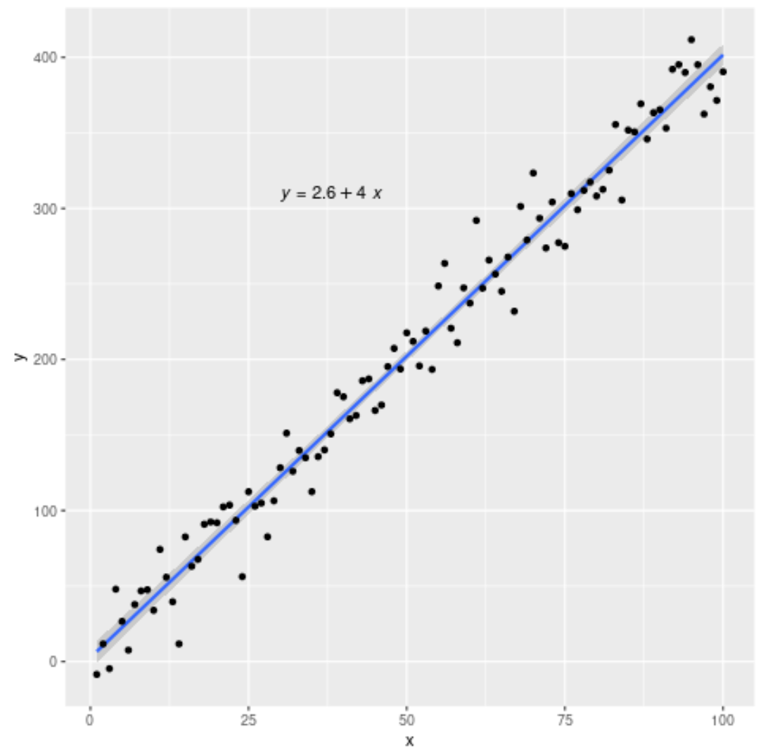
接下来，我们将使用以下语法创建具有拟合回归线和方程的散点图：

 #load necessary libraries
library (ggplot2)
library (ggpubr)

#create plot with regression line and regression equation
ggplot(data=df, aes (x=x, y=y)) +
        geom_smooth(method=" lm ") +
        geom_point() +
        stat_regline_equation(label. x =30, label. y =310) 

这告诉我们拟合的回归方程是：

y = 2.6 + 4*(x)

请注意， label.x和label.y指定要显示的回归方程的 (x,y) 坐标。

步骤 3：将 R 方添加到图中（可选）

如果您想使用以下语法，还可以添加回归模型的 R 平方值：

 #load necessary libraries
library (ggplot2)
library (ggpubr)

#create plot with regression line, regression equation, and R-squared
ggplot(data=df, aes (x=x, y=y)) +
        geom_smooth(method=" lm ") +
        geom_point() +
        stat_regline_equation(label. x =30, label. y =310) +
stat_cor( aes (label=..rr.label..), label. x =30, label. y =290) 

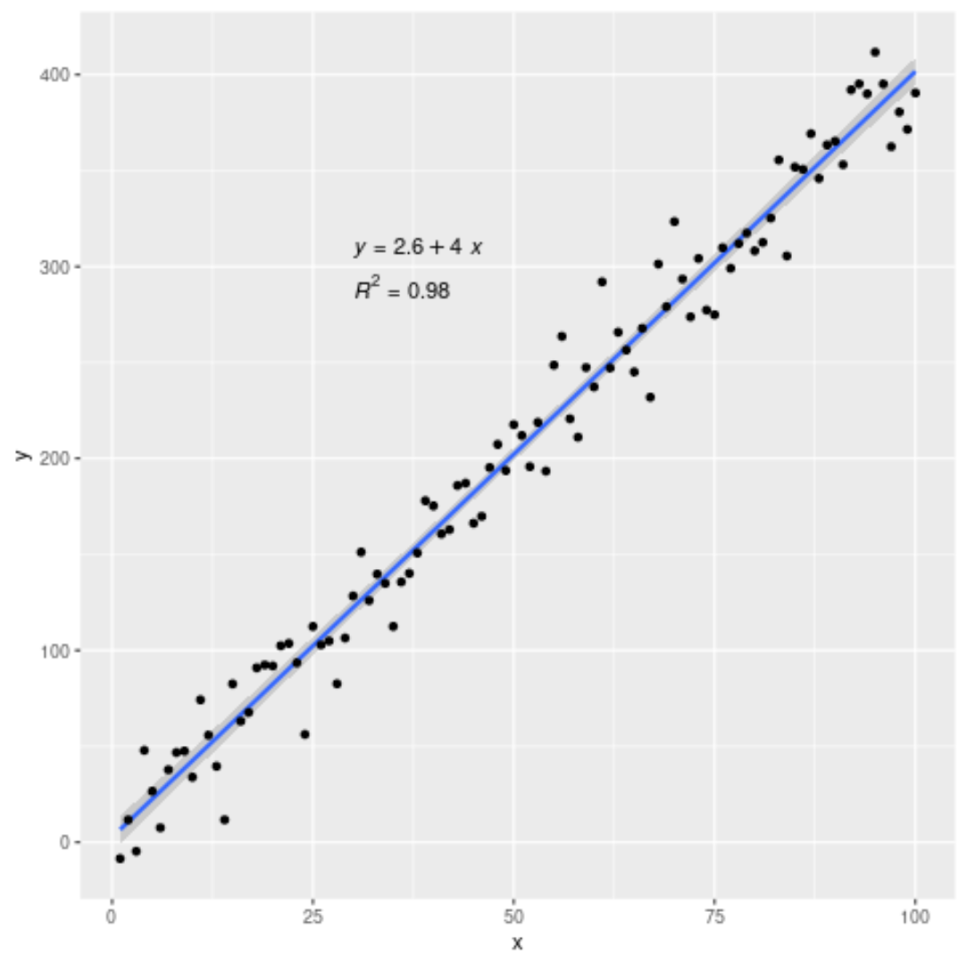
该模型的R 平方结果为0.98 。

您可以在此页面上找到更多 R 教程。