如何在 r 中执行 mann-kendall 趋势检验

Mann-Kendall 趋势检验用于确定时间序列数据是否存在趋势。这是非参数检验，意味着不对数据的正态性做出任何基本假设。

检验假设如下：

H ₀ （零假设）：数据中不存在趋势。

H _A （替代假设）：数据中存在趋势。 （这可能是积极的或消极的趋势）

如果检验的 p 值低于一定的显着性水平（常见选择为 0.10、0.05 和 0.01），则有统计显着性证据表明时间序列数据中存在趋势。

本教程介绍如何在 R 中执行 Mann-Kendall 趋势检验。

示例：R 中的 Mann-Kendall 趋势检验

要在 R 中执行 Mann-Kendall 趋势检验，我们将使用Kendall库中的MannKendall()函数，该函数使用以下语法：

曼肯德尔(x)

金子：

• x = 数据向量，通常是时间序列

为了说明如何执行测试，我们将使用Kendall图书馆的内置PrecipGL数据集，其中包含 1900 年至 1986 年所有五大湖的年降水量信息：

 #load Kendall library and PrecipGL dataset
library(Kendall)
data(PrecipGL)

#view dataset
PrecipGL

Time Series:
Start = 1900 
End = 1986 
Frequency = 1 
[1] 31.69 29.77 31.70 33.06 31.31 32.72 31.18 29.90 29.17 31.48 28.11 32.61
[13] 31.31 30.96 28.40 30.68 33.67 28.65 30.62 30.21 28.79 30.92 30.92 28.13
[25] 30.51 27.63 34.80 32.10 33.86 32.33 25.69 30.60 32.85 30.31 27.71 30.34
[37] 29.14 33.41 33.51 29.90 32.69 32.34 35.01 33.05 31.15 36.36 29.83 33.70
[49] 29.81 32.41 35.90 37.45 30.39 31.15 35.75 31.14 30.06 32.40 28.44 36.38
[61] 31.73 31.27 28.51 26.01 31.27 35.57 30.85 33.35 35.82 31.78 34.25 31.43
[73] 35.97 33.87 28.94 34.62 31.06 38.84 32.25 35.86 32.93 32.69 34.39 33.97
[85] 32.15 40.16 36.32
attr(,"title")
[1] Annual precipitation, 1900-1986, Entire Great Lakes

要查看数据是否存在趋势，我们可以进行Mann-Kendall趋势检验：

 #Perform the Mann-Kendall Trend Test
MannKendall(PrecipGL)

tau = 0.265, 2-sided pvalue = 0.00029206

检验统计量为0.265 ，相应的双尾 p 值为0.00029206 。由于该 p 值小于 0.05，我们将拒绝检验的原假设并得出数据中存在趋势的结论。

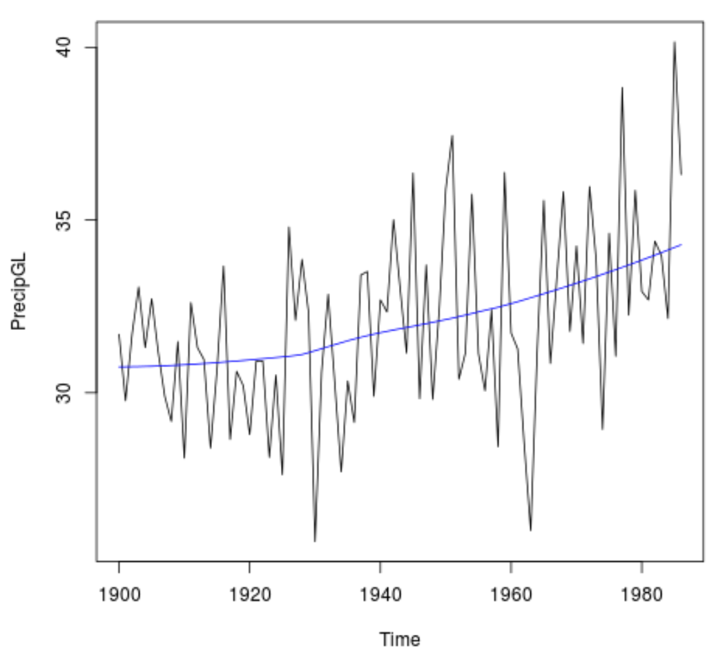
为了可视化趋势，我们可以创建每年降水量的时间图，并添加一条平滑线来表示趋势：

 #Plot the time series data
plot(PrecipGL)

#Add a smooth line to visualize the trend 
lines(lowess(time(PrecipGL),PrecipGL), col='blue')

请注意，我们还可以使用SeasonalMannKendall(x)命令执行季节性调整的 Mann-Kendall 趋势检验，以解释数据中的任何季节性：

 #Perform a seasonally-adjusted Mann-Kendall Trend Test
SeasonalMannKendall(PrecipGL)

tau = 0.265, 2-sided pvalue = 0.00028797

检验统计量为0.265 ，相应的双尾 p 值为0.00028797 。该 p 值再次小于 0.05，因此我们将拒绝检验的原假设并得出数据中存在趋势的结论。