आर में एलएम() परिणाम कैसे प्लॉट करें

आप R में lm() फ़ंक्शन के परिणामों को प्लॉट करने के लिए निम्नलिखित विधियों का उपयोग कर सकते हैं:

विधि 1: प्लॉट एलएम () का परिणाम आधार आर है

 #create scatterplot
plot(y ~ x, data=data)

#add fitted regression line to scatterplot
abline(fit)

विधि 2: प्लॉट lm() का परिणाम ggplot2 होता है

 library (ggplot2)

#create scatterplot with fitted regression line
ggplot(data, aes (x = x, y = y)) + 
  geom_point() +
  stat_smooth(method = " lm ")

निम्नलिखित उदाहरण दिखाते हैं कि आर में निर्मित एमटीकार्स डेटासेट के साथ अभ्यास में प्रत्येक विधि का उपयोग कैसे करें।

उदाहरण 1: प्लॉट एलएम() का परिणाम आधार आर है

निम्नलिखित कोड दिखाता है कि बेस आर में एलएम() फ़ंक्शन के परिणामों को कैसे प्लॉट किया जाए:

 #fit regression model
fit <- lm(mpg ~ wt, data=mtcars)

#create scatterplot
plot(mpg ~ wt, data=mtcars)

#add fitted regression line to scatterplot
abline(fit) 

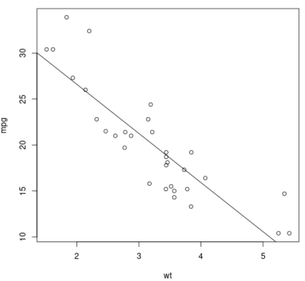
ग्राफ़ में बिंदु कच्चे डेटा मानों का प्रतिनिधित्व करते हैं और सीधी विकर्ण रेखा फिट प्रतिगमन रेखा का प्रतिनिधित्व करती है।

उदाहरण 2: प्लॉट एलएम() परिणाम जीजीप्लॉट2 में

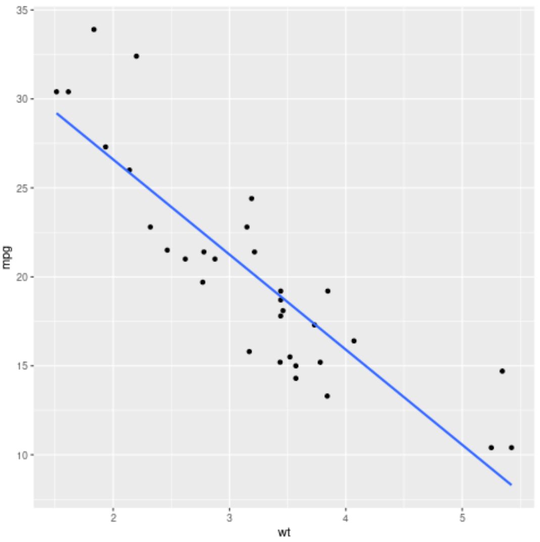
निम्नलिखित कोड दिखाता है कि ggplot2 डेटा विज़ुअलाइज़ेशन पैकेज का उपयोग करके lm() फ़ंक्शन के परिणामों को कैसे प्लॉट किया जाए:

 library (ggplot2)

#fit regression model
fit <- lm(mpg ~ wt, data=mtcars)

#create scatterplot with fitted regression line
ggplot(mtcars, aes (x = x, y = y)) +
  geom_point() +
  stat_smooth(method = " lm ")

नीली रेखा फिट प्रतिगमन रेखा का प्रतिनिधित्व करती है और ग्रे बैंड 95% विश्वास अंतराल की सीमा का प्रतिनिधित्व करते हैं।

विश्वास अंतराल सीमा को हटाने के लिए, बस stat_smooth() तर्क में se=FALSE का उपयोग करें:

 library (ggplot2) 

#fit regression model
fit <- lm(mpg ~ wt, data=mtcars)

#create scatterplot with fitted regression line
ggplot(mtcars, aes (x = x, y = y)) +
  geom_point() +
  stat_smooth(method = “ lm ”, se= FALSE ) 

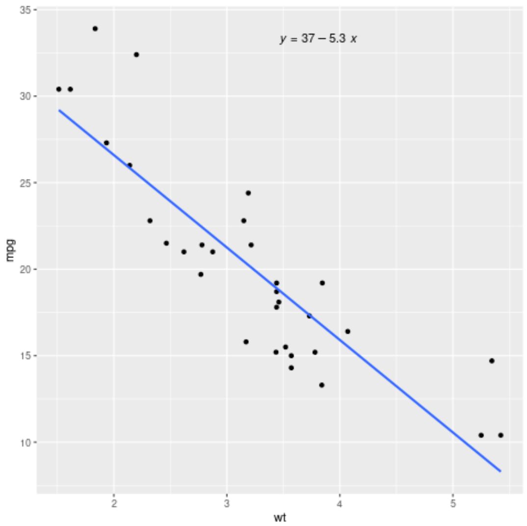
आप ggpubr पैकेज से stat_regline_equation() फ़ंक्शन का उपयोग करके ग्राफ़ के अंदर फिटेड रिग्रेशन समीकरण भी जोड़ सकते हैं:

 library (ggplot2)
library (ggpubr)

#fit regression model
fit <- lm(mpg ~ wt, data=mtcars)

#create scatterplot with fitted regression line
ggplot(mtcars, aes (x = x, y = y)) +
  geom_point() +
  stat_smooth(method = “ lm ”, se= FALSE ) +
  stat_regline_equation(label.x.npc = “ center ”) 

अतिरिक्त संसाधन

निम्नलिखित ट्यूटोरियल बताते हैं कि आर में अन्य सामान्य कार्य कैसे करें:

आर में सरल रैखिक प्रतिगमन कैसे करें
आर में प्रतिगमन आउटपुट की व्याख्या कैसे करें
आर में जीएलएम और एलएम के बीच अंतर