पायथन में बेल कर्व कैसे बनाएं

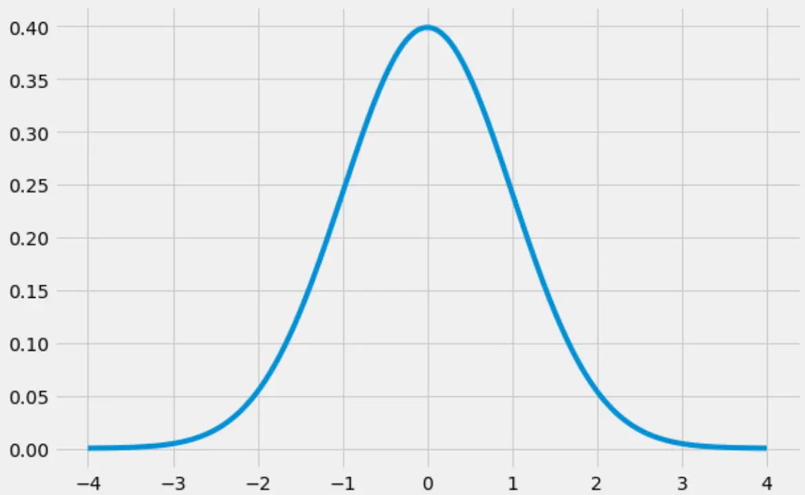
“घंटी वक्र” एक सामान्य वितरण के आकार को दिया गया उपनाम है , जिसका एक विशिष्ट “घंटी” आकार होता है:

यह ट्यूटोरियल बताता है कि पायथन में बेल कर्व कैसे बनाया जाता है।

पायथन में बेल कर्व कैसे बनाएं

निम्नलिखित कोड दिखाता है कि numpy , scipy और matplotlib लाइब्रेरीज़ का उपयोग करके घंटी वक्र कैसे बनाया जाए:

 import numpy as np
import matplotlib.pyplot as plt
from scipy.stats import norm

#create range of x-values from -4 to 4 in increments of .001
x = np.arange(-4, 4, 0.001)

#create range of y-values that correspond to normal pdf with mean=0 and sd=1 
y = norm.pdf(x,0,1)

#defineplot 
fig, ax = plt.subplots(figsize=(9,6))
ax.plot(x,y)

#choose plot style and display the bell curve 
plt.style.use('fivethirtyeight')
plt.show() 

पायथन में बेल कर्व कैसे भरें

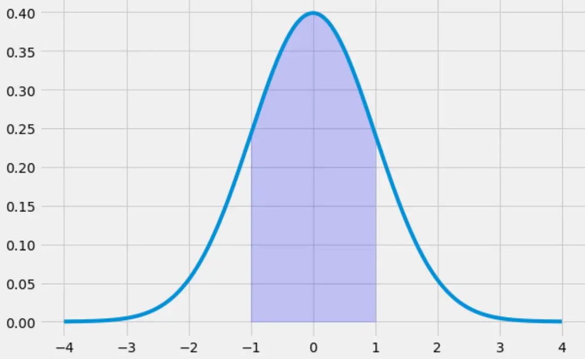
निम्नलिखित कोड दर्शाता है कि -1 से 1 तक जाने वाले घंटी वक्र के नीचे के क्षेत्र को कैसे भरें:

 x = np.arange(-4, 4, 0.001)
y = norm.pdf(x,0,1)

fig, ax = plt.subplots(figsize=(9,6))
ax.plot(x,y)

#specify the region of the bell curve to fill in 
x_fill = np.arange(-1, 1, 0.001)
y_fill = norm.pdf(x_fill,0,1)
ax.fill_between(x_fill,y_fill,0, alpha=0.2, color='blue')

plt.style.use('fivethirtyeight')
plt.show() 

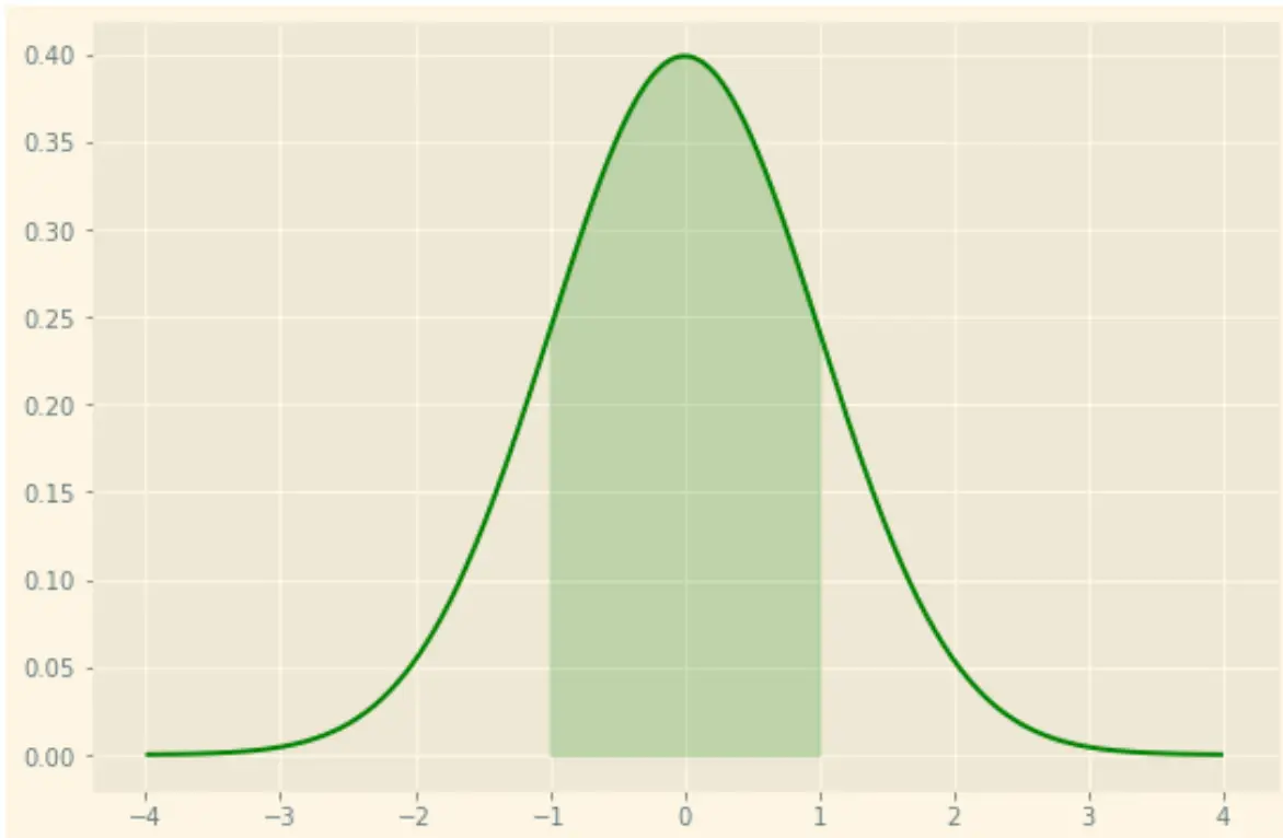
ध्यान दें कि आप matplotlib के कई स्टाइलिंग विकल्पों का उपयोग करके प्लॉट को अपनी इच्छानुसार स्टाइल भी कर सकते हैं। उदाहरण के लिए, आप हरी रेखा और हरी छायांकन के साथ “सूरज की रोशनी” थीम का उपयोग कर सकते हैं:

 x = np.arange(-4, 4, 0.001)
y = norm.pdf(x,0,1)

fig, ax = plt.subplots(figsize=(9,6))
ax.plot(x,y, color=' green ')

#specify the region of the bell curve to fill in 
x_fill = np.arange(-1, 1, 0.001)
y_fill = norm.pdf(x_fill,0,1)
ax.fill_between(x_fill,y_fill,0, alpha=0.2, color=' green ')

plt.style.use(' Solarize_Light2 ')
plt.show() 

आप matplotlib के लिए संपूर्ण स्टाइलशीट संदर्भ मार्गदर्शिका यहां पा सकते हैं।

अतिरिक्त संसाधन

एक्सेल में बेल कर्व कैसे बनाएं