Python での曲線近似 (例付き)

Python でデータセットに曲線を当てはめたい場合がよくあります。

次のステップバイステップの例では、Python でnumpy.polyfit()関数を使用して曲線をデータに適合させる方法と、どの曲線がデータに最も適合するかを判断する方法を説明します。

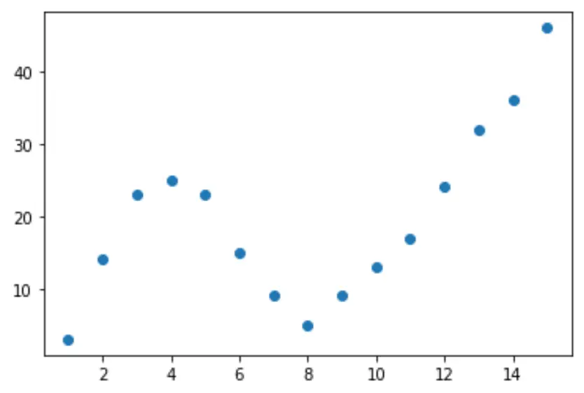
ステップ 1: データの作成と視覚化

まず偽のデータセットを作成し、次に散布図を作成してデータを視覚化しましょう。

 import pandas as pd
import matplotlib. pyplot as plt

#createDataFrame
df = pd. DataFrame ({' x ': [1, 2, 3, 4, 5, 6, 7, 8, 9, 10, 11, 12, 13, 14, 15],
                   ' y ': [3, 14, 23, 25, 23, 15, 9, 5, 9, 13, 17, 24, 32, 36, 46]})

#create scatterplot of x vs. y
plt. scatter (df. x , df. y ) 

ステップ 2: 複数のカーブを調整する

次に、いくつかの多項式回帰モデルをデータに適合させ、同じプロットで各モデルの曲線を視覚化してみましょう。

 import numpy as np

#fit polynomial models up to degree 5
model1 = np. poly1d (np. polyfit (df. x , df. y , 1))
model2 = np. poly1d (np. polyfit (df. x , df. y , 2))
model3 = np. poly1d (np. polyfit (df. x , df. y , 3))
model4 = np. poly1d (np. polyfit (df. x , df. y , 4))
model5 = np. poly1d (np. polyfit (df. x , df. y , 5))

#create scatterplot
polyline = np. linspace (1, 15, 50)
plt. scatter (df. x , df. y )

#add fitted polynomial lines to scatterplot 
plt. plot (polyline, model1(polyline), color=' green ')
plt. plot (polyline, model2(polyline), color=' red ')
plt. plot (polyline, model3(polyline), color=' purple ')
plt. plot (polyline, model4(polyline), color=' blue ')
plt. plot (polyline, model5(polyline), color=' orange ')
plt. show ()

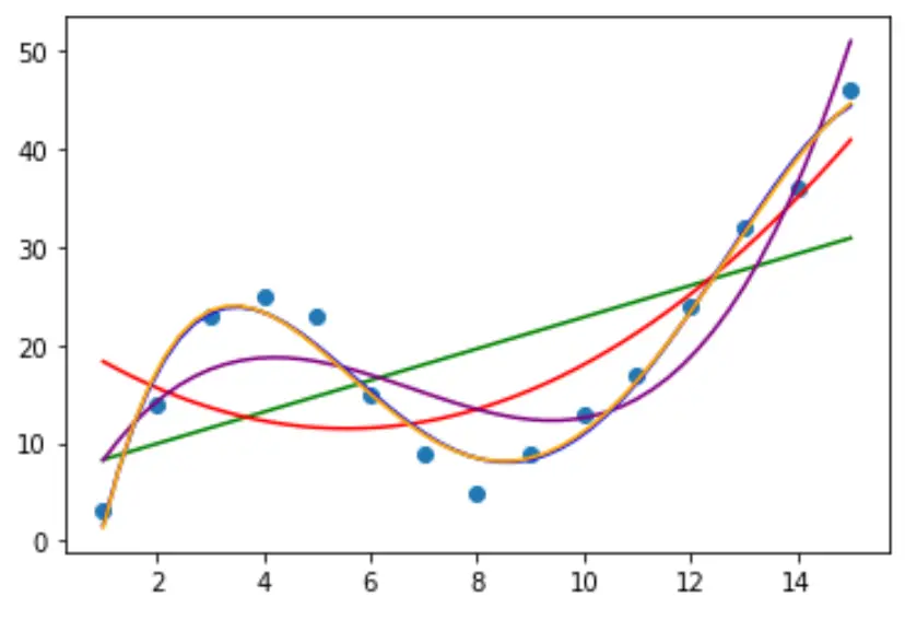
どの曲線がデータに最もよく適合するかを判断するには、各モデルの調整された R 二乗を確認します。

この値は、予測変数の数を調整した、モデル内の予測変数によって説明できる応答変数の変動のパーセンテージを示します。

 #define function to calculate adjusted r-squared
def adjR(x, y, degree):
    results = {}
    coeffs = np. polyfit (x, y, degree)
    p = np. poly1d (coeffs)
    yhat = p(x)
    ybar = np. sum (y)/len(y)
    ssreg = np. sum ((yhat-ybar)**2)
    sstot = np. sum ((y - ybar)**2)
    results[' r_squared '] = 1- (((1-(ssreg/sstot))*(len(y)-1))/(len(y)-degree-1))

    return results

#calculated adjusted R-squared of each model
adjR(df. x , df. y , 1)
adjR(df. x , df. y , 2)
adjR(df. x , df. y , 3)
adjR(df. x , df. y , 4)
adjR(df. x , df. y , 5)

{'r_squared': 0.3144819}
{'r_squared': 0.5186706}
{'r_squared': 0.7842864}
{'r_squared': 0.9590276}
{'r_squared': 0.9549709}

結果から、調整された R 二乗が最も高いモデルは、調整された R 二乗が0.959である 4 次多項式であることがわかります。

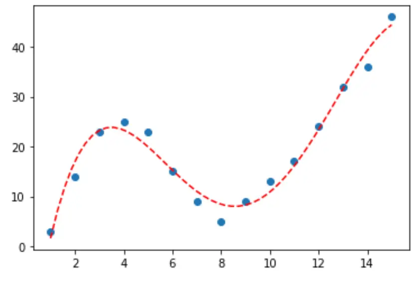
ステップ 3: 最終的な曲線を視覚化する

最後に、4 次多項式モデルの曲線を使用して散布図を作成できます。

 #fit fourth-degree polynomial
model4 = np. poly1d (np. polyfit (df. x , df. y , 4))

#define scatterplot
polyline = np. linspace (1, 15, 50)
plt. scatter (df. x , df. y )

#add fitted polynomial curve to scatterplot
plt. plot (polyline, model4(polyline), ' -- ', color=' red ')
plt. show ()

print()関数を使用して、この行の方程式を取得することもできます。

 print (model4)

          4 3 2
-0.01924x + 0.7081x - 8.365x + 35.82x - 26.52

曲線の方程式は次のとおりです。

y = -0.01924x ⁴ + 0.7081x ³ – 8.365x ² + 35.82x – 26.52

この方程式を使用すると、モデル内の予測変数に基づいて応答変数の値を予測できます。たとえば、 x = 4 の場合、 y = 23.32と予測します。

y = -0.0192(4) ⁴ + 0.7081(4) ³ – 8.365(4) ² + 35.82(4) – 26.52 = 23.32

追加リソース

多項式回帰の概要
Python で多項式回帰を実行する方法