Python で多次元スケーリングを実行する方法

統計学では、多次元スケーリングは、抽象的なデカルト空間 (通常は 2D 空間) 内のデータ セット内の観察の類似性を視覚化する方法です。

Python で多次元スケーリングを実行する最も簡単な方法は、 sklearn.manifoldサブモジュールのMDS()関数を使用することです。

次の例は、この関数を実際に使用する方法を示しています。

例: Python での多次元スケーリング

さまざまなバスケットボール選手に関する情報を含む次のパンダ データフレームがあるとします。

 import pandas as pd

#create DataFrane
df = pd. DataFrame ({' player ': ['A', 'B', 'C', 'D', 'E', 'F', 'G', 'H', 'I', 'J', 'K '],
                   ' points ': [4, 4, 6, 7, 8, 14, 16, 19, 25, 25, 28],
                   ' assists ': [3, 2, 2, 5, 4, 8, 7, 6, 8, 10, 11],
                   ' blocks ': [7, 3, 6, 7, 5, 8, 8, 4, 2, 2, 1],
                   ' rebounds ': [4, 5, 5, 6, 5, 8, 10, 4, 3, 2, 2]})

#set player column as index column
df = df. set_index (' player ')

#view Dataframe
print (df)

        points assists blocks rebounds
player                                   
A 4 3 7 4
B 4 2 3 5
C 6 2 6 5
D 7 5 7 6
E 8 4 5 5
F 14 8 8 8
G 16 7 8 10
H 19 6 4 4
I 25 8 2 3
D 25 10 2 2
K 28 11 1 2

次のコードを使用して、 sklearn.manifoldモジュールのMDS()関数で多次元スケーリングを実行できます。

 from sklearn. manifold import MDS

#perform multi-dimensional scaling
mds = MDS(random_state= 0 )
scaled_df = mds. fit_transform (df)

#view results of multi-dimensional scaling
print (scaled_df)

[[ 7.43654469 8.10247222]
 [4.13193821 10.27360901]
 [5.20534681 7.46919526]
 [6.22323046 4.45148627]
 [3.74110999 5.25591459]
 [3.69073384 -2.88017811]
 [3.89092087 -5.19100988]
 [ -3.68593169 -3.0821144 ]
 [ -9.13631889 -6.81016012]
 [ -8.97898385 -8.50414387]
 [-12.51859044 -9.08507097]]

元の DataFrame の各行は、(x, y) 座標に縮小されています。

次のコードを使用して、これらの座標を 2D 空間で視覚化できます。

 import matplotlib.pyplot as plt

#create scatterplot
plt. scatter (scaled_df[:,0], scaled_df[:,1])

#add axis labels
plt. xlabel (' Coordinate 1 ')
plt. ylabel (' Coordinate 2 ')

#add lables to each point
for i, txt in enumerate( df.index ):
    plt. annotate (txt, (scaled_df[:,0][i]+.3, scaled_df[:,1][i]))

#display scatterplot
plt. show ()

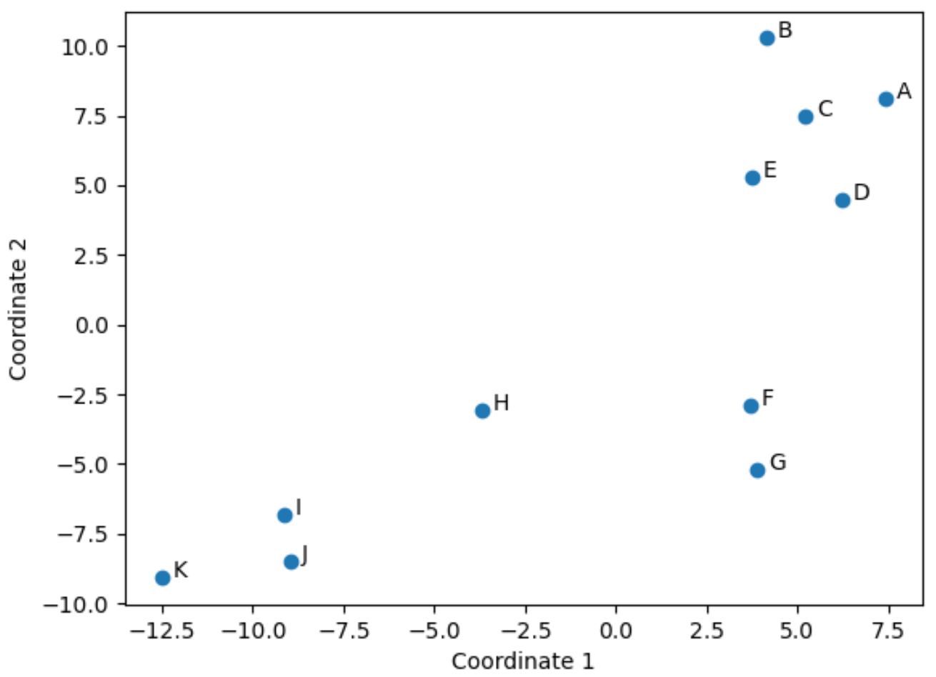
元のデータフレーム内の、元の 4 つの列 (ポイント、アシスト、ブロック、リバウンド) の値が類似しているプレーヤーは、プロット内で互いに近くにあります。

たとえば、プレーヤーFとGは互いに接近しています。元の DataFrame の値は次のとおりです。

 #select rows with index labels 'F' and 'G'
df. loc [[' F ',' G ']]

        points assists blocks rebounds
player				
F 14 8 8 8
G 16 7 8 10

ポイント、アシスト、ブロック、リバウンドの値はすべて非常に似ており、2D プロットでそれらが互いに非常に近い理由が説明されています。

対照的に、プロット内で遠く離れたプレーヤーBとKについて考えてみましょう。

元の DataFrame でそれらの値を参照すると、それらがまったく異なることがわかります。

 #select rows with index labels 'B' and 'K'
df. loc [[' B ',' K ']]

        points assists blocks rebounds
player				
B 4 2 3 5
K 28 11 1 2

したがって、2D プロットは、DataFframe 内のすべての変数にわたって各プレーヤーがどの程度類似しているかを視覚化するのに適した方法です。

プロット内では、同様の統計情報を持つプレイヤーは近くにグループ化されますが、非常に異なる統計情報を持つプレイヤーは互いに遠く離れています。

追加リソース

次のチュートリアルでは、Python で他の一般的なタスクを実行する方法について説明します。

Python でデータを正規化する方法
Python で外れ値を削除する方法
Python で正規性をテストする方法