Python での線形判別分析 (ステップバイステップ)

線形判別分析は、一連の予測子変数があり、 応答変数を2 つ以上のクラスに分類する場合に使用できる方法です。

このチュートリアルでは、Python で線形判別分析を実行する方法の例を段階的に説明します。

ステップ 1: 必要なライブラリをロードする

まず、この例に必要な関数とライブラリをロードします。

 from sklearn. model_selection import train_test_split
from sklearn. model_selection import RepeatedStratifiedKFold
from sklearn. model_selection import cross_val_score
from sklearn. discriminant_analysis import LinearDiscriminantAnalysis 
from sklearn import datasets
import matplotlib. pyplot as plt
import pandas as pd
import numpy as np

ステップ 2: データをロードする

この例では、sklearn ライブラリのirisデータセットを使用します。次のコードは、このデータセットをロードし、使いやすいように pandas DataFrame に変換する方法を示しています。

 #load iris dataset
iris = datasets. load_iris ()

#convert dataset to pandas DataFrame
df = pd.DataFrame(data = np.c_[iris[' data '], iris[' target ']],
                 columns = iris[' feature_names '] + [' target '])
df[' species '] = pd. Categorical . from_codes (iris.target, iris.target_names)
df.columns = [' s_length ', ' s_width ', ' p_length ', ' p_width ', ' target ', ' species ']

#view first six rows of DataFrame
df. head ()

   s_length s_width p_length p_width target species
0 5.1 3.5 1.4 0.2 0.0 setosa
1 4.9 3.0 1.4 0.2 0.0 setosa
2 4.7 3.2 1.3 0.2 0.0 setosa
3 4.6 3.1 1.5 0.2 0.0 setosa
4 5.0 3.6 1.4 0.2 0.0 setosa

#find how many total observations are in dataset
len( df.index )

150

データセットには合計 150 個の観測値が含まれていることがわかります。

この例では、特定の花がどの種に属するかを分類するための線形判別分析モデルを構築します。

モデルでは次の予測子変数を使用します。

• がく片の長さ
• がく片の幅
• 花びらの長さ
• 花びらの幅

そして、それらを使用して、次の 3 つの潜在的なクラスをサポートする種の応答変数を予測します。

• セトサ
• 癜風
• バージニア州

ステップ 3: LDA モデルを調整する

次に、sklearn のLinearDiscriminantAnalsys関数を使用して、LDA モデルをデータに適合させます。

 #define predictor and response variables
X = df[[' s_length ',' s_width ',' p_length ',' p_width ']]
y = df[' species ']

#Fit the LDA model
model = LinearDiscriminantAnalysis()
model. fit (x,y)

ステップ 4: モデルを使用して予測を行う

データを使用してモデルをフィッティングしたら、層別 k 分割交差検証を繰り返してモデルのパフォーマンスを評価できます。

この例では、10 回の折り目と 3 回の繰り返しを使用します。

 #Define method to evaluate model
cv = RepeatedStratifiedKFold(n_splits= 10 , n_repeats= 3 , random_state= 1 )

#evaluate model
scores = cross_val_score(model, X, y, scoring=' accuracy ', cv=cv, n_jobs=-1)
print( np.mean (scores))  

0.9777777777777779

モデルが97.78%の平均精度を達成したことがわかります。

このモデルを使用して、入力値に基づいて新しい花がどのクラスに属するかを予測することもできます。

 #define new observation
new = [5, 3, 1, .4]

#predict which class the new observation belongs to
model. predict ([new])

array(['setosa'], dtype='<U10')

このモデルは、この新しい観測結果がsetosaと呼ばれる種に属することを予測していることがわかります。

ステップ 5: 結果を視覚化する

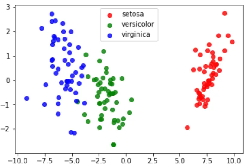
最後に、LDA プロットを作成してモデルの線形判別式を視覚化し、データセット内の 3 つの異なる種をどの程度分離しているかを視覚化できます。

 #define data to plot
X = iris.data
y = iris.target
model = LinearDiscriminantAnalysis()
data_plot = model. fit (x,y). transform (X)
target_names = iris. target_names

#create LDA plot
plt. figure ()
colors = [' red ', ' green ', ' blue ']
lw = 2
for color, i, target_name in zip(colors, [0, 1, 2], target_names):
    plt. scatter (data_plot[y == i, 0], data_plot[y == i, 1], alpha=.8, color=color,
                label=target_name)

#add legend to plot
plt. legend (loc=' best ', shadow= False , scatterpoints=1)

#display LDA plot
plt. show ()

このチュートリアルで使用される完全な Python コードは、 ここで見つけることができます。