Lm() の結果を r にプロットする方法
次のメソッドを使用して、R のlm()関数の結果をプロットできます。
方法 1: lm() の結果を基数 R でプロットする
 #create scatterplot
plot(y ~ x, data=data)

#add fitted regression line to scatterplot
abline(fit)
方法 2: lm() の結果を ggplot2 にプロットする
 library (ggplot2)

#create scatterplot with fitted regression line
ggplot(data, aes (x = x, y = y)) +
  geom_point() +
  stat_smooth(method = " lm ")
次の例は、R に組み込まれているmtcars データセットを使用して各メソッドを実際に使用する方法を示しています。
例 1: lm() の結果の基数 R をプロットする
次のコードは、 lm()関数の結果を基数 R でプロットする方法を示しています。
 #fit regression model
fit <- lm(mpg ~ wt, data=mtcars)

#create scatterplot
plot(mpg ~ wt, data=mtcars)

#add fitted regression line to scatterplot
abline(fit)
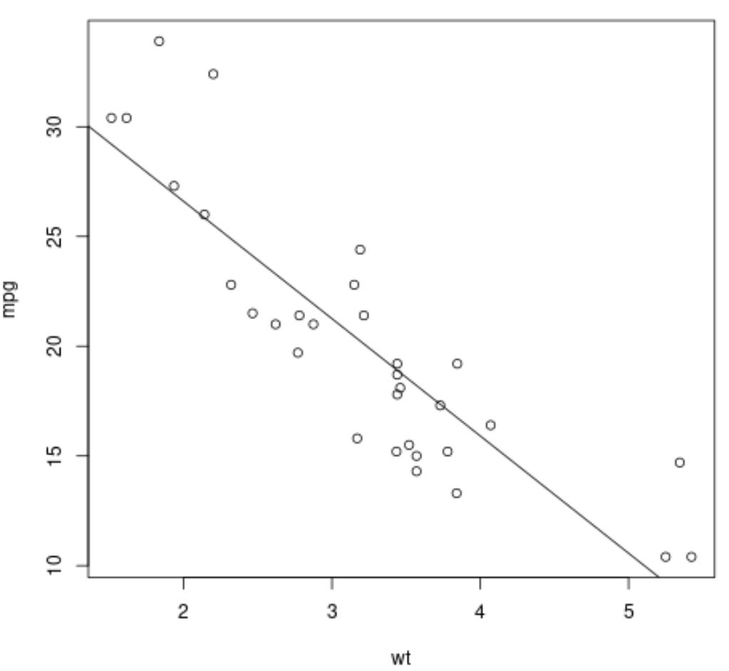
グラフ内の点は生データ値を表し、直線の対角線は近似された回帰直線を表します。
例 2: lm() の結果を ggplot2 にプロットする
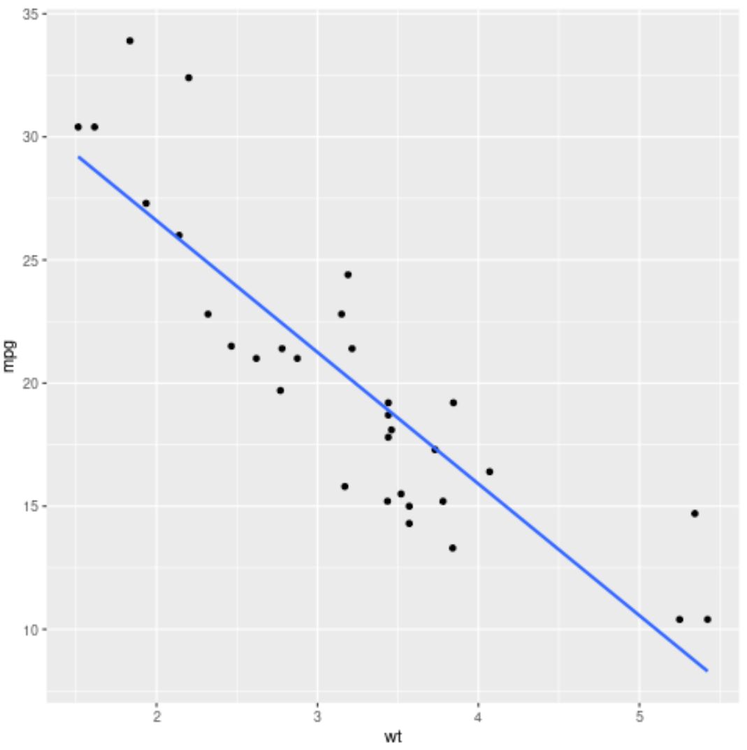
次のコードは、 ggplot2データ視覚化パッケージを使用してlm()関数の結果をプロットする方法を示しています。
 library (ggplot2)

#fit regression model
fit <- lm(mpg ~ wt, data=mtcars)

#create scatterplot with fitted regression line
ggplot(mtcars, aes (x = x, y = y)) +
  geom_point() +
  stat_smooth(method = " lm ")

青い線は近似された回帰直線を表し、灰色のバンドは 95% 信頼区間の限界を表します。
信頼区間の境界を削除するには、 stat_smooth()引数でse=FALSEを使用するだけです。
 library (ggplot2)

#fit regression model
fit <- lm(mpg ~ wt, data=mtcars)

#create scatterplot with fitted regression line
ggplot(mtcars, aes (x = x, y = y)) +
  geom_point() +
  stat_smooth(method = “ lm ”, se= FALSE )
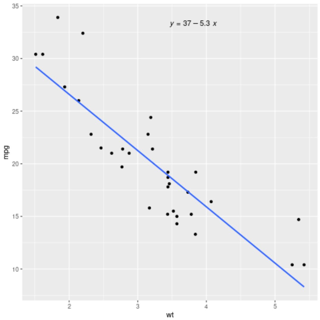
ggpubrパッケージのstat_regline_equation()関数を使用して、近似回帰式をグラフ内に追加することもできます。
 library (ggplot2)
library (ggpubr)

#fit regression model
fit <- lm(mpg ~ wt, data=mtcars)

#create scatterplot with fitted regression line
ggplot(mtcars, aes (x = x, y = y)) +
  geom_point() +
  stat_smooth(method = “ lm ”, se= FALSE ) +
  stat_regline_equation(label.x.npc = “ center ”)
追加リソース
次のチュートリアルでは、R で他の一般的なタスクを実行する方法について説明します。
著者について
ベンジャミン・アンダーソン博士
私はベンジャミンです。退職した統計教授から、専任の Statorials 教育者になりました。 統計分野における豊富な経験と専門知識を活かして、私は Statorials を通じて学生に力を与えるために自分の知識を共有することに尽力しています。もっと知る