R で多項式回帰曲線をプロットする方法

多項式回帰は、予測変数と応答変数の間の関係が非線形である場合に使用する回帰手法です。

このチュートリアルでは、R で多項式回帰曲線をプロットする方法を説明します。

関連:最も一般的な 7 種類の回帰

例: R での多項式回帰曲線のプロット

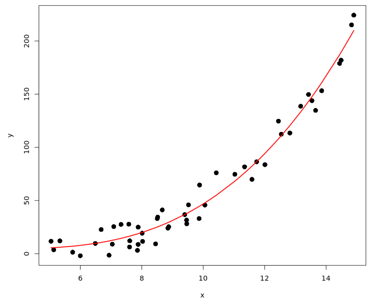
次のコードは、多項式回帰モデルをデータセットに近似し、散布図の生データに多項式回帰曲線をプロットする方法を示しています。

 #define data
x <- runif(50, 5, 15)
y <- 0.1*x^3 - 0.5 * x^2 - x + 5 + rnorm(length(x),0,10) 
 
#plot x vs. y
plot(x, y, pch= 16 , cex= 1.5 ) 
 
#fit polynomial regression model
fit <- lm(y ~ x + I(x^2) + I(x^3))
 
#use model to get predicted values
pred <- predict(fit)
ix <- sort(x, index. return = T )$ix

#add polynomial curve to plot
lines(x[ix], pred[ix], col=' red ', lwd= 2 )

text()関数を使用して、近似された多項式回帰方程式をプロットに追加することもできます。

 #define data
x <- runif(50, 5, 15)
y <- 0.1*x^3 - 0.5 * x^2 - x + 5 + rnorm(length(x),0,10) 
 
#plot x vs. y
plot(x, y, pch=16, cex=1.5) 
 
#fit polynomial regression model
fit <- lm(y ~ x + I(x^2) + I(x^3))
 
#use model to get predicted values
pred <- predict(fit)
ix <- sort(x, index. return = T )$ix

#add polynomial curve to plot
lines(x[ix], pred[ix], col=' red ', lwd= 2 )

#get model coefficients
coeff <- round(fit$coefficients, 2)

#add fitted model equation to plot
text(9, 200 , paste("Model: ", coeff[1], " + ", coeff[2],
                    "*x", "+", coeff[3], "*x^2", "+", coeff[4], "*x^3"), cex= 1.3 )

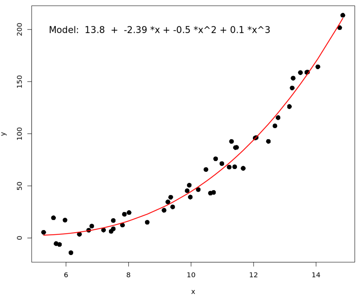
cex引数はテキストのフォント サイズを制御することに注意してください。デフォルトは 1 なので、テキストを読みやすくするために値1.3を使用することにしました。

追加リソース

多項式回帰の概要
Excel で多項式曲線を近似する方法
Python で多項式回帰を実行する方法