R で dffits を計算する方法

統計では、さまざまな観測値が回帰モデルにどのような影響を与えるかを知りたいことがよくあります。

観測値の影響を計算する 1 つの方法は、「適合度の差」を表すDFFITSとして知られる指標を使用することです。

このメトリクスは、個々の観測値を省略したときに回帰モデルによる予測がどの程度変化するかを示します。

このチュートリアルでは、R のモデル内の各観測値の DFFITS を計算して視覚化する方法の段階的な例を示します。

ステップ 1: 回帰モデルを作成する

まず、R に組み込まれているmtcarsデータセットを使用して重線形回帰モデルを作成します。

 #load the dataset
data(mtcars)

#fit a regression model
model <- lm(mpg~disp+hp, data=mtcars)

#view model summary
summary(model)

Coefficients:
             Estimate Std. Error t value Pr(>|t|)    
(Intercept) 30.735904 1.331566 23.083 < 2nd-16 ***
available -0.030346 0.007405 -4.098 0.000306 ***
hp -0.024840 0.013385 -1.856 0.073679 .  
---
Significant. codes: 0 '***' 0.001 '**' 0.01 '*' 0.05 '.' 0.1 ' ' 1

Residual standard error: 3.127 on 29 degrees of freedom
Multiple R-squared: 0.7482, Adjusted R-squared: 0.7309 
F-statistic: 43.09 on 2 and 29 DF, p-value: 2.062e-09

ステップ 2: 各観測値の DFFITS を計算する

次に、組み込みのdffits()関数を使用して、モデル内の各観測値の DFFITS 値を計算します。

 #calculate DFFITS for each observation in the model
dffits <- as . data . frame (dffits(model))

#display DFFITS for each observation
challenges

                    dffits(model)
Mazda RX4 -0.14633456
Mazda RX4 Wag -0.14633456
Datsun 710 -0.19956440
Hornet 4 Drive 0.11540062
Hornet Sportabout 0.32140303
Valiant -0.26586716
Duster 360 0.06282342
Merc 240D -0.03521572
Merc 230 -0.09780612
Merc 280 -0.22680622
Merc 280C -0.32763355
Merc 450SE -0.09682952
Merc 450SL -0.03841129
Merc 450SLC -0.17618948
Cadillac Fleetwood -0.15860270
Lincoln Continental -0.15567627
Chrysler Imperial 0.39098449
Fiat 128 0.60265798
Honda Civic 0.35544919
Toyota Corolla 0.78230167
Toyota Corona -0.25804885
Dodge Challenger -0.16674639
AMC Javelin -0.20965432
Camaro Z28 -0.08062828
Pontiac Firebird 0.67858692
Fiat X1-9 0.05951528
Porsche 914-2 0.09453310
Lotus Europa 0.55650363
Ford Pantera L 0.31169050
Ferrari Dino -0.29539098
Maserati Bora 0.76464932
Volvo 142E -0.24266054

通常、閾値 2√ p/nを超える DFFITS 値の観測値を詳しく調べます。

• p:モデルで使用される予測変数の数
• n:モデルで使用される観測値の数

この例では、しきい値は0.5になります。

 #find number of predictors in model
p <- length (model$coefficients)-1

#find number of observations
n <- nrow (mtcars)

#calculate DFFITS threshold value
thresh <- 2* sqrt (p/n)

thresh

[1] 0.5

DFFITS 値に基づいて観測値を並べ替えて、それらのいずれかがしきい値を超えているかどうかを確認できます。

 #sort observations by DFFITS, descending
dffits[ order (-dffits[' dffits(model) ']), ]

 [1] 0.78230167 0.76464932 0.67858692 0.60265798 0.55650363 0.39098449
 [7] 0.35544919 0.32140303 0.31169050 0.11540062 0.09453310 0.06282342
[13] 0.05951528 -0.03521572 -0.03841129 -0.08062828 -0.09682952 -0.09780612
[19] -0.14633456 -0.14633456 -0.15567627 -0.15860270 -0.16674639 -0.17618948
[25] -0.19956440 -0.20965432 -0.22680622 -0.24266054 -0.25804885 -0.26586716
[31] -0.29539098 -0.32763355

最初の 5 つの観測値の DFFITS 値が 0.5 より大きいことがわかります。これは、これらの観測値がモデルに大きな影響を与えているかどうかを判断するために、これらの観測値をより詳しく調査する必要があることを意味します。

ステップ 3: 各観測値の DFFITS を視覚化する

最後に、各観測値の DFFITS を視覚化する簡単なグラフを作成できます。

 #plot DFFITS values for each observation
plot(dffits(model), type = ' h ')

#add horizontal lines at absolute values for threshold
abline(h = thresh, lty = 2)
abline(h = -thresh, lty = 2)

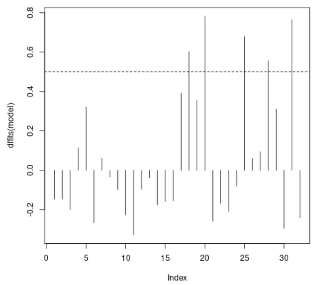
X 軸はデータセット内の各観測値のインデックスを表示し、Y 値は各観測値に対応する DFFITS 値を表示します。

追加リソース

R で単純な線形回帰を実行する方法
R で重回帰を実行する方法
R でレバレッジ統計を計算する方法
R で残差プロットを作成する方法