R에서 부트스트래핑하는 방법(예제 포함)

부트스트래핑은 통계 의 표준 오차를 추정하고 통계에 대한 신뢰 구간을 생성하는 데 사용할 수 있는 방법입니다.

부트스트래핑의 기본 프로세스는 다음과 같습니다.

• 주어진 데이터 세트에서 k개의 반복 샘플을 복원하여 추출합니다.
• 각 샘플에 대해 관심 있는 통계를 계산합니다.
• 이는 주어진 통계에 대해 k 개의 서로 다른 추정치를 제공하며, 이를 사용하여 통계의 표준 오차를 계산하고 통계에 대한 신뢰 구간을 생성할 수 있습니다.

부트스트랩 라이브러리 의 다음 함수를 사용하여 R에서 부트스트랩을 수행할 수 있습니다.

1. 부트스트랩 샘플을 생성합니다.

boot(데이터, 통계, R, …)

금:

• 데이터: 벡터, 행렬 또는 데이터 블록
• 통계: 시작할 통계를 생성하는 함수
• A: 부트스트랩 반복 횟수

2. 부트스트랩 신뢰 구간을 생성합니다.

boot.ci(부팅 개체, conf, 유형)

금:

• bootobject: boot() 함수에 의해 반환된 객체
• conf: 계산할 신뢰 구간입니다. 기본값은 0.95입니다.
• 유형: 계산할 신뢰 구간 유형입니다. 옵션에는 ‘standard’, ‘basic’, ‘stud’, ‘perc’, ‘bca’ 및 ‘all’이 포함되며 기본값은 ‘all’입니다.

다음 예에서는 이러한 기능을 실제로 사용하는 방법을 보여줍니다.

예 1: 단일 통계 부트스트랩

다음 코드는 단순 선형 회귀 모델의 R 제곱 에 대한 표준 오차를 계산하는 방법을 보여줍니다.

 set.seed(0)
library (boot)

#define function to calculate R-squared
rsq_function <- function (formula, data, indices) {
  d <- data[indices,] #allows boot to select sample
  fit <- lm(formula, data=d) #fit regression model
  return (summary(fit)$r.square) #return R-squared of model
}
#perform bootstrapping with 2000 replications
reps <- boot(data=mtcars, statistic=rsq_function, R=2000, formula=mpg~disp)

#view results of boostrapping
reps

ORDINARY NONPARAMETRIC BOOTSTRAP


Call:
boot(data = mtcars, statistic = rsq_function, R = 2000, formula = mpg ~ 
    available)


Bootstrap Statistics:
     original bias std. error
t1* 0.7183433 0.002164339 0.06513426

결과에서 다음을 확인할 수 있습니다.

• 이 회귀 모델의 추정 R-제곱은 0.7183433 입니다.
• 이 추정치의 표준 오류는 0.06513426 입니다.

또한 부트스트랩된 샘플의 분포를 빠르게 시각화할 수 있습니다.

 plot(reps)

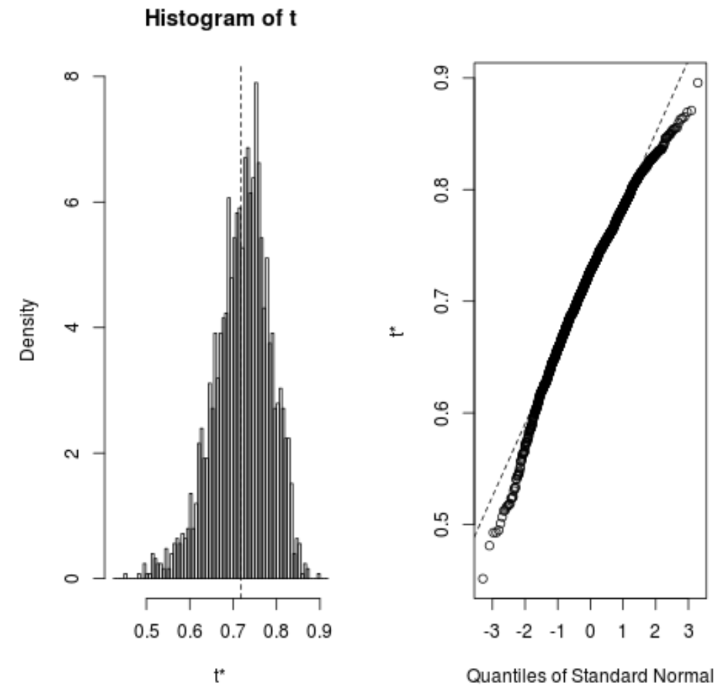
다음 코드를 사용하여 모델의 추정 R 제곱에 대한 95% 신뢰 구간을 계산할 수도 있습니다.

 #calculate adjusted bootstrap percentile (BCa) interval
boot.ci(reps, type=" bca ")

CALL: 
boot.ci(boot.out = reps, type = "bca")

Intervals: 
Level BCa          
95% (0.5350, 0.8188)  
Calculations and Intervals on Original Scale

결과에서 실제 R-제곱 값에 대한 부트스트랩된 95% 신뢰 구간은 (0.5350, 0.8188)임을 알 수 있습니다.

예 2: 부트스트랩 다중 통계

다음 코드는 다중 선형 회귀 모델의 각 계수에 대한 표준 오차를 계산하는 방법을 보여줍니다.

 set.seed(0)
library (boot)

#define function to calculate fitted regression coefficients
coef_function <- function (formula, data, indices) {
  d <- data[indices,] #allows boot to select sample
  fit <- lm(formula, data=d) #fit regression model
  return (coef(fit)) #return coefficient estimates of model
}

#perform bootstrapping with 2000 replications
reps <- boot(data=mtcars, statistic=coef_function, R=2000, formula=mpg~disp)

#view results of boostrapping
reps

ORDINARY NONPARAMETRIC BOOTSTRAP


Call:
boot(data = mtcars, statistic = coef_function, R = 2000, formula = mpg ~ 
    available)


Bootstrap Statistics:
       original bias std. error
t1* 29.59985476 -5.058601e-02 1.49354577
t2* -0.04121512 6.549384e-05 0.00527082

결과에서 다음을 확인할 수 있습니다.

• 모델 절편의 추정 계수는 29.59985476 이고 이 추정의 표준 오차는 1.49354577 입니다.
• 모델의 예측 변수 disp 에 대한 추정 계수는 -0.04121512 이고 이 추정의 표준 오차는 0.00527082 입니다.

또한 부트스트랩된 샘플의 분포를 빠르게 시각화할 수 있습니다.

 plot(reps, index=1) #intercept of model
plot(reps, index=2) #disp predictor variable

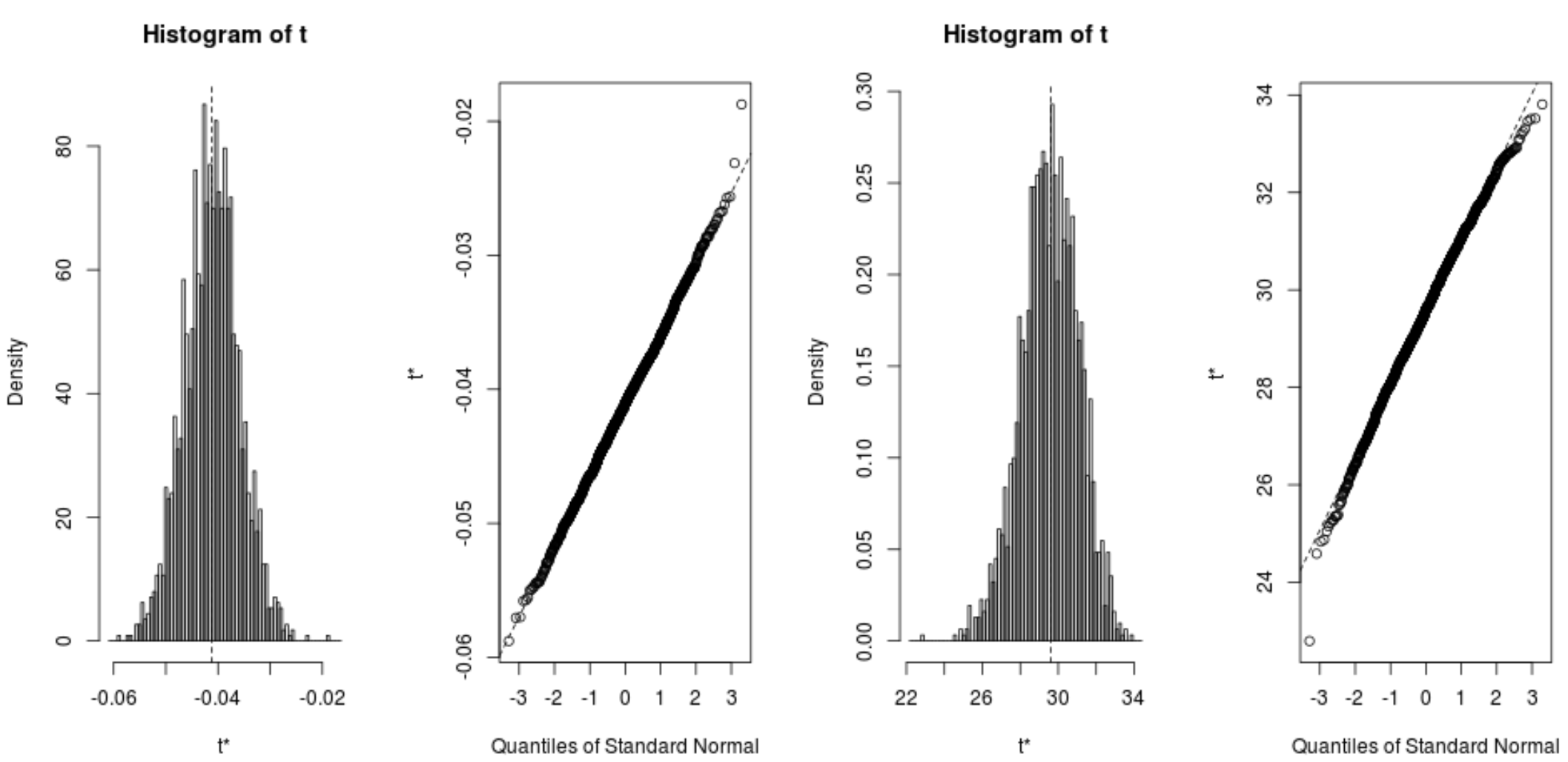
다음 코드를 사용하여 각 계수에 대한 95% 신뢰 구간을 계산할 수도 있습니다.

 #calculate adjusted bootstrap percentile (BCa) intervals
boot.ci(reps, type=" bca ", index=1) #intercept of model
boot.ci(reps, type=" bca ", index=2) #disp predictor variable

CALL: 
boot.ci(boot.out = reps, type = "bca", index = 1)

Intervals: 
Level BCa          
95% (26.78, 32.66)  
Calculations and Intervals on Original Scale
BOOTSTRAP CONFIDENCE INTERVAL CALCULATIONS
Based on 2000 bootstrap replicates

CALL: 
boot.ci(boot.out = reps, type = "bca", index = 2)

Intervals: 
Level BCa          
95% (-0.0520, -0.0312)  
Calculations and Intervals on Original Scale

결과에서 모델 계수에 대한 부트스트래핑된 95% 신뢰 구간은 다음과 같음을 알 수 있습니다.

• 차단용 IC: (26.78, 32.66)
• disp 용 CI : (-.0520, -.0312)

추가 리소스

R에서 단순 선형 회귀를 수행하는 방법
R에서 다중 선형 회귀를 수행하는 방법
신뢰 구간 소개