R의 플롯에 회귀 방정식을 추가하는 방법

종종 다음과 같이 R의 플롯에 회귀 방정식을 추가할 수 있습니다.

다행히도 ggplot2 및 ggpubr 패키지의 기능을 사용하면 매우 쉽게 수행할 수 있습니다.

이 튜토리얼에서는 이러한 패키지의 함수를 사용하여 R의 플롯에 회귀 방정식을 추가하는 방법에 대한 단계별 예를 제공합니다.

1단계: 데이터 생성

먼저 작업할 가짜 데이터를 만들어 보겠습니다.

 #make this example reproducible
set. seeds (1)

#create data frame
df <- data. frame (x = c(1:100))
df$y <- 4*df$x + rnorm(100, sd=20)

#view head of data frame
head(df)

  xy
1 1 -8.529076
2 2 11.672866
3 3 -4.712572
4 4 47.905616
5 5 26.590155
6 6 7.590632

2단계: 회귀 방정식을 사용하여 플롯 만들기

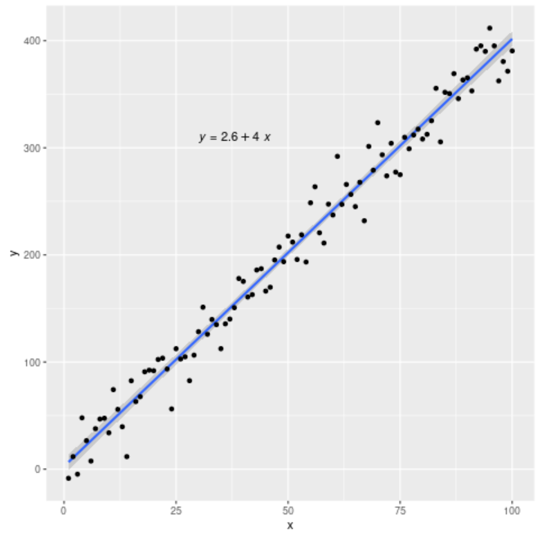
다음으로 다음 구문을 사용하여 적합 회귀선과 방정식이 포함된 산점도를 만듭니다.

 #load necessary libraries
library (ggplot2)
library (ggpubr)

#create plot with regression line and regression equation
ggplot(data=df, aes (x=x, y=y)) +
        geom_smooth(method=" lm ") +
        geom_point() +
        stat_regline_equation(label. x =30, label. y =310) 

이는 적합 회귀 방정식이 다음과 같다는 것을 알려줍니다.

y = 2.6 + 4*(x)

label.x 및 label.y는 표시할 회귀 방정식의 (x,y) 좌표를 지정합니다.

3단계: 플롯에 R-제곱 추가(선택 사항)

다음 구문을 사용하려는 경우 회귀 모델의 R 제곱 값을 추가할 수도 있습니다.

 #load necessary libraries
library (ggplot2)
library (ggpubr)

#create plot with regression line, regression equation, and R-squared
ggplot(data=df, aes (x=x, y=y)) +
        geom_smooth(method=" lm ") +
        geom_point() +
        stat_regline_equation(label. x =30, label. y =310) +
stat_cor( aes (label=..rr.label..), label. x =30, label. y =290) 

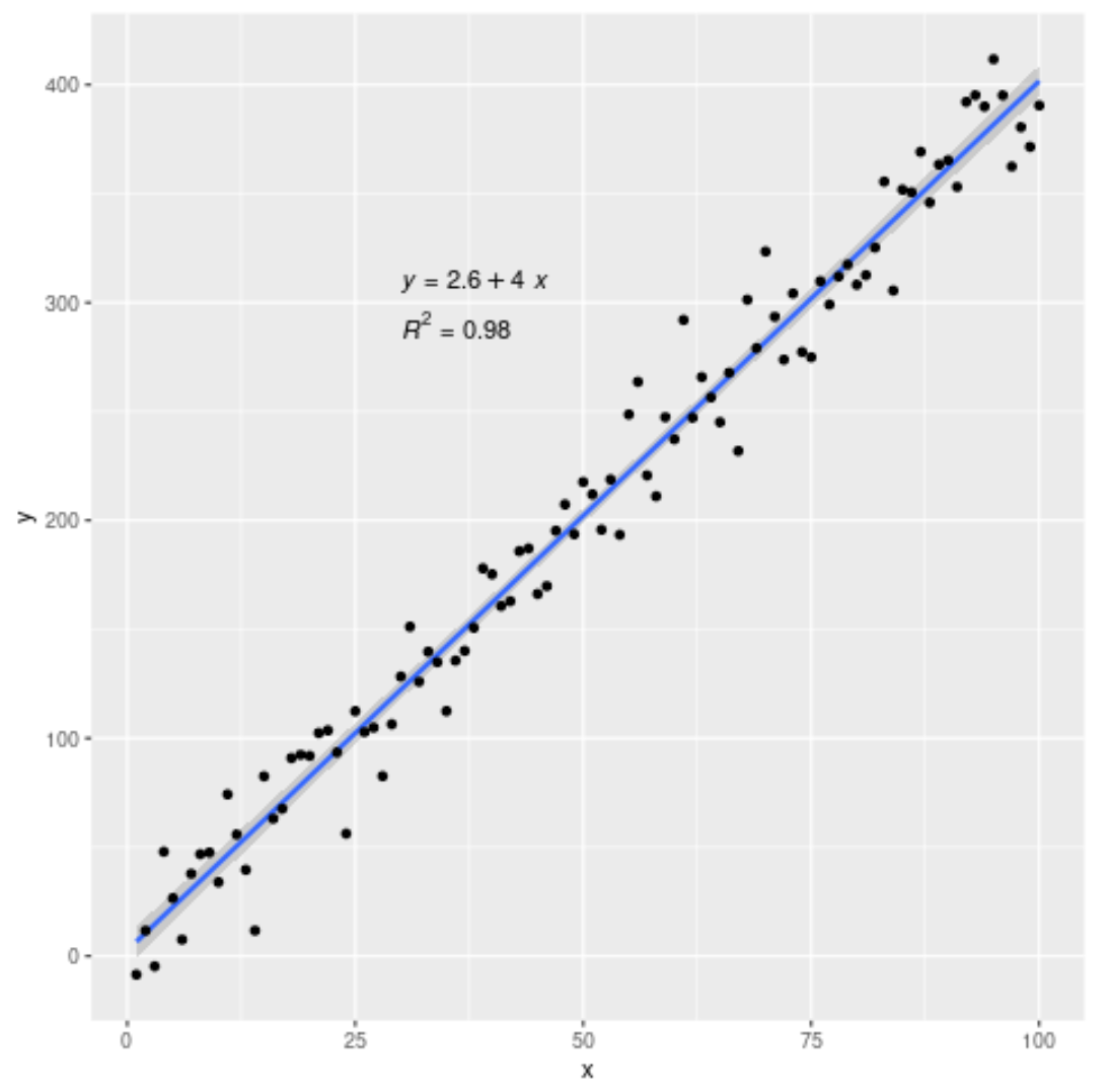
이 모델의 R-제곱은 0.98 로 나타났습니다.

이 페이지 에서 더 많은 R 튜토리얼을 찾을 수 있습니다.