Python에서 여러 roc 곡선을 그리는 방법(예제 포함)

기계 학습에서 분류 모델 의 성능을 시각화하는 한 가지 방법은 “수신기 작동 특성” 곡선을 나타내는 ROC 곡선을 만드는 것입니다.

종종 여러 분류 모델을 단일 데이터 세트에 맞추고 각 모델에 대한 ROC 곡선을 만들어 어떤 모델이 데이터에서 가장 잘 작동하는지 시각화할 수 있습니다.

다음 단계별 예제에서는 Python에서 여러 ROC 곡선을 그리는 방법을 보여줍니다.

1단계: 필요한 패키지 가져오기

먼저, 몇 가지 필수 패키지를 Python으로 가져옵니다.

 from sklearn import metrics
from sklearn import datasets
from sklearn. model_selection import train_test_split
from sklearn. linear_model import LogisticRegression
from sklearn. set import GradientBoostingClassifier
import numpy as np
import matplotlib. pyplot as plt

2단계: 가짜 데이터 생성

다음으로 sklearn의 make_classification() 함수를 사용하여 1000개의 행, 4개의 예측 변수 및 이진 응답 변수가 있는 가짜 데이터 세트를 만듭니다.

 #create fake dataset
X, y = datasets. make_classification (n_samples= 1000 ,
                                    n_features= 4 ,
                                    n_informative= 3 ,
                                    n_redundant= 1 ,
                                    random_state= 0 )

#split dataset into training and testing set
X_train, X_test, y_train, y_test = train_test_split(X, y, test_size= .3 , random_state= 0 )

3단계: 여러 모델을 피팅하고 ROC 곡선 그리기

다음으로, 로지스틱 회귀 모델을 적용한 다음 경사 강화 모델을 데이터에 적용하고 동일한 플롯에 각 모델에 대한 ROC 곡선을 그립니다.

 #set up plotting area
plt. Figure (0). clf ()

#fit logistic regression model and plot ROC curve
model = LogisticRegression()
model. fit (X_train, y_train)
y_pred = model. predict_proba (X_test)[:, 1]
fpr, tpr, _ = metrics. roc_curve (y_test, y_pred)
auc = round(metrics. roc_auc_score (y_test, y_pred), 4)
plt. plot (fpr,tpr,label="Logistic Regression, AUC="+str(auc))

#fit gradient boosted model and plot ROC curve
model = GradientBoostingClassifier()
model. fit (X_train, y_train)
y_pred = model. predict_proba (X_test)[:, 1]
fpr, tpr, _ = metrics. roc_curve (y_test, y_pred)
auc = round(metrics. roc_auc_score (y_test, y_pred), 4)
plt. plot (fpr,tpr,label="Gradient Boosting, AUC="+str(auc))

#add legend
plt. legend () 

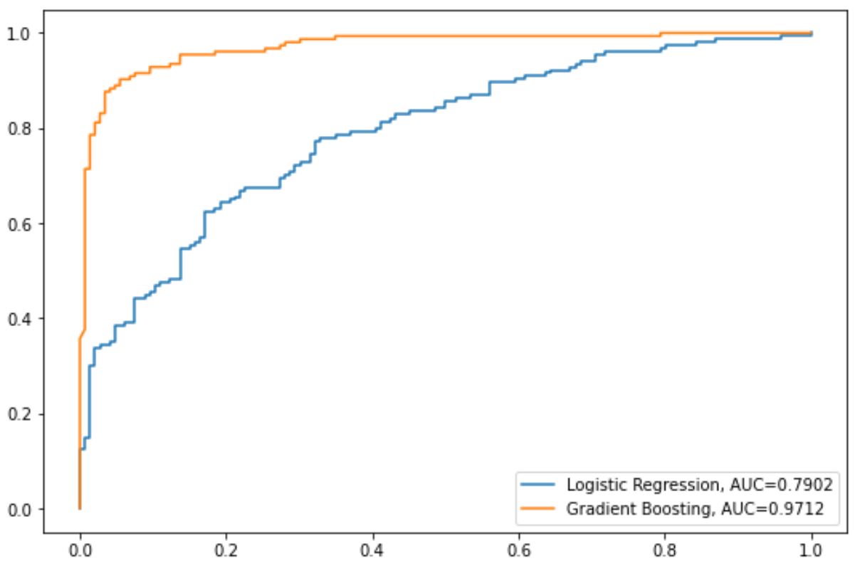
파란색 선은 로지스틱 회귀 모델의 ROC 곡선을 나타내고 주황색 선은 그래디언트 부스팅 모델의 ROC 곡선을 나타냅니다.

ROC 곡선이 플롯의 왼쪽 상단 모서리에 가까울수록 모델이 데이터를 범주로 더 잘 분류할 수 있습니다.

이를 정량화하기 위해 곡선 아래에 있는 플롯의 양을 알려주는 AUC(곡선 아래 영역)를 계산할 수 있습니다.

AUC가 1에 가까울수록 모델이 더 좋습니다.

차트에서 각 모델에 대한 다음 AUC 측정항목을 볼 수 있습니다.

• 로지스틱 회귀 모델의 AUC: 0.7902
• 경사 강화 모델의 AUC: 0.9712

분명히 경사 강화 모델은 로지스틱 회귀 모델보다 데이터를 범주로 분류하는 데 더 성공적입니다.

추가 리소스

다음 자습서에서는 분류 모델 및 ROC 곡선에 대한 추가 정보를 제공합니다.

로지스틱 회귀 소개
ROC 곡선을 해석하는 방법(예제 포함)
좋은 AUC 점수는 무엇입니까?