Python တွင် linear discriminant analysis (အဆင့်ဆင့်)
တစ်ပြေးညီ ခွဲခြားမှု ခွဲခြမ်းစိတ်ဖြာခြင်း သည် သင့်တွင် ကြိုတင်ခန့်မှန်းကိန်းရှင်များ အစုတစ်ခုရှိ၍ တုံ့ပြန်မှုကိန်းရှင်ကို အတန်းနှစ်ခု သို့မဟုတ် ထို့ထက်ပိုသော အတန်းအစားများအဖြစ် ခွဲခြားလိုသောအခါတွင် သင်သုံးနိုင်သော နည်းလမ်းတစ်ခုဖြစ်သည်။
ဤသင်ခန်းစာသည် Python တွင် linear discriminant analysis ပြုလုပ်ပုံအဆင့်ဆင့်ကို ဥပမာပေးပါသည်။
အဆင့် 1- လိုအပ်သောစာကြည့်တိုက်များကို တင်ပါ။
ဦးစွာ၊ ဤဥပမာအတွက် လိုအပ်သော လုပ်ဆောင်ချက်များနှင့် ဒစ်ဂျစ်တိုက်များကို တင်ပေးပါမည်။
 from sklearn. model_selection import train_test_split
from sklearn. model_selection import RepeatedStratifiedKFold
from sklearn. model_selection import cross_val_score
from sklearn. discriminant_analysis import LinearDiscriminantAnalysis
from sklearn import datasets
import matplotlib. pyplot as plt
import pandas as pd
import numpy as np
အဆင့် 2: ဒေတာကို တင်ပါ။
ဤဥပမာအတွက်၊ ကျွန်ုပ်တို့သည် sklearn စာကြည့်တိုက်မှ iris dataset ကို အသုံးပြုပါမည်။ အောက်ပါကုဒ်သည် ဤဒေတာအတွဲကို မည်သို့တင်ရမည်ကို ပြသပြီး အသုံးပြုရလွယ်ကူစေရန် ပန်ဒါ DataFrame အဖြစ်သို့ ပြောင်းနိုင်သည်-
 #load iris dataset
iris = datasets. load_iris ()

#convert dataset to pandas DataFrame
df = pd.DataFrame(data = np.c_[iris[' data '], iris[' target ']],
                 columns = iris[' feature_names '] + [' target '])
df[' species '] = pd. Categorical . from_codes (iris.target, iris.target_names)
df.columns = [' s_length ', ' s_width ', ' p_length ', ' p_width ', ' target ', ' species ']

#view first six rows of DataFrame
df. head ()

   s_length s_width p_length p_width target species
0 5.1 3.5 1.4 0.2 0.0 setosa
1 4.9 3.0 1.4 0.2 0.0 setosa
2 4.7 3.2 1.3 0.2 0.0 setosa
3 4.6 3.1 1.5 0.2 0.0 setosa
4 5.0 3.6 1.4 0.2 0.0 setosa

#find how many total observations are in dataset
len( df.index )

150
ဒေတာအတွဲတွင် စူးစမ်းမှုပေါင်း ၁၅၀ ပါဝင်ကြောင်း ကျွန်ုပ်တို့တွေ့မြင်နိုင်ပါသည်။
ဤဥပမာအတွက်၊ ပေးထားသောပန်းအမျိုးအစားကို အမျိုးအစားခွဲခြားရန် linear discriminant analysis model တစ်ခုကို တည်ဆောက်ပါမည်။
ကျွန်ုပ်တို့သည် မော်ဒယ်တွင် အောက်ပါ ကြိုတင်ခန့်မှန်းကိန်းရှင်များကို အသုံးပြုပါမည်-
- နှုတ်ခမ်းသားအရှည်
- Sepal အကျယ်
- ပွင့်ချပ်အရှည်
- ပွင့်ချပ်အကျယ်
အောက်ဖော်ပြပါ ဖြစ်နိုင်ချေရှိသော အတန်းသုံးမျိုးအား ပံ့ပိုးပေးသည့် Species response variable ကို ခန့်မှန်းရန် ၎င်းတို့ကို အသုံးပြုပါမည်။
- setosa
- စွယ်စုံရောင်
- ဗာဂျီးနီးယား
အဆင့် 3- LDA မော်ဒယ်ကို ချိန်ညှိပါ။
ထို့နောက်၊ ကျွန်ုပ်တို့သည် sklearn ၏ LinearDiscriminantAnalsys လုပ်ဆောင်ချက်ကို အသုံးပြု၍ ကျွန်ုပ်တို့၏ဒေတာနှင့် LDA မော်ဒယ်ကို အံကိုက်လုပ်ပါမည်။
 #define predictor and response variables
X = df[[' s_length ',' s_width ',' p_length ',' p_width ']]
y = df[' species ']

#Fit the LDA model
model = LinearDiscriminantAnalysis()
model. fit (x,y)
အဆင့် 4- ခန့်မှန်းချက်များကို ပြုလုပ်ရန် မော်ဒယ်ကို အသုံးပြုပါ။
ကျွန်ုပ်တို့၏ဒေတာကိုအသုံးပြု၍ မော်ဒယ်ကို တပ်ဆင်ပြီးသည်နှင့်၊ ထပ်ခါတလဲလဲ stratified k-fold cross-validation ကို အသုံးပြု၍ မော်ဒယ်၏စွမ်းဆောင်ရည်ကို အကဲဖြတ်နိုင်ပါသည်။
ဤဥပမာအတွက်၊ ကျွန်ုပ်တို့သည် 10 ခေါက်နှင့် ထပ်ခါတလဲလဲ 3 ခုကို အသုံးပြုပါမည်။
 #Define method to evaluate model
cv = RepeatedStratifiedKFold(n_splits= 10 , n_repeats= 3 , random_state= 1 )

#evaluate model
scores = cross_val_score(model, X, y, scoring=' accuracy ', cv=cv, n_jobs=-1)
print( np.mean (scores))

0.9777777777777779
မော်ဒယ်သည် ပျမ်းမျှတိကျမှု 97.78% ရရှိသည်ကို ကျွန်ုပ်တို့တွေ့မြင်နိုင်ပါသည်။
ထည့်သွင်းတန်ဖိုးများကို အခြေခံ၍ ပန်းအသစ်တစ်ခု၏ အတန်းအစား မည်သည့်အမျိုးအစားဖြစ်သည်ကို ခန့်မှန်းရန် မော်ဒယ်ကိုလည်း အသုံးပြုနိုင်သည်။
 #define new observation
new = [5, 3, 1, .4]

#predict which class the new observation belongs to
model. predict ([new])

array(['setosa'], dtype='<U10')
ဤလေ့လာတွေ့ရှိချက်အသစ်သည် setosa ဟုခေါ်သောမျိုးစိတ်များနှင့်သက်ဆိုင်ကြောင်း မော်ဒယ်က ခန့်မှန်းသည်ကို ကျွန်ုပ်တို့တွေ့မြင်ရပါသည်။
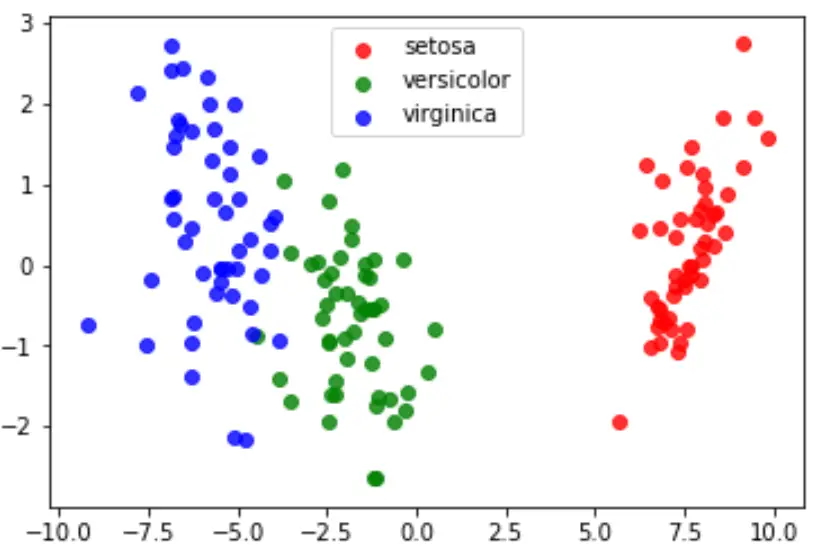
အဆင့် 5- ရလဒ်များကို မြင်ယောင်ကြည့်ပါ။
နောက်ဆုံးတွင်၊ ကျွန်ုပ်တို့သည် မော်ဒယ်၏ တစ်ပြေးညီ ခွဲခြားဆက်ဆံမှုများကို မြင်သာစေရန် LDA ကြံစည်မှုကို ဖန်တီးနိုင်ပြီး ကျွန်ုပ်တို့၏ဒေတာအတွဲတွင် မတူညီသောမျိုးစိတ်သုံးမျိုးကို မည်မျှကောင်းစွာ ပိုင်းခြားထားသည်ကို မြင်ယောင်နိုင်သည်-
 #define data to plot
X = iris.data
y = iris.target
model = LinearDiscriminantAnalysis()
data_plot = model. fit (x,y). transform (X)
target_names = iris. target_names

#create LDA plot
plt. figure ()
colors = [' red ', ' green ', ' blue ']
lw = 2
for color, i, target_name in zip(colors, [0, 1, 2], target_names):
    plt. scatter (data_plot[y == i, 0], data_plot[y == i, 1], alpha=.8, color=color,
                label=target_name)

#add legend to plot
plt. legend (loc=' best ', shadow= False , scatterpoints=1)

#display LDA plot
plt. show ()
ဤသင်ခန်းစာတွင်အသုံးပြုထားသော Python ကုဒ်အပြည့်အစုံကို ဤနေရာတွင် ရှာတွေ့နိုင်ပါသည်။
စာရေးသူအကြောင်း
Benjamin Anderson
မင်္ဂလာပါ၊ ကျွန်ုပ်သည် အငြိမ်းစား စာရင်းအင်း ပါမောက္ခ ဘင်ဂျမင်ဖြစ်ပြီး သီးသန့် Statorials ဆရာအဖြစ် လှည့်ပတ်ပါသည်။ စာရင်းဇယားနယ်ပယ်တွင် ကျယ်ပြန့်သောအတွေ့အကြုံနှင့် ကျွမ်းကျင်မှုနှင့်အတူ၊ Statorials မှတစ်ဆင့် ကျောင်းသားများကို ခွန်အားဖြစ်စေရန်အတွက် ကျွန်ုပ်၏အသိပညာကို မျှဝေလိုပါသည်။ ပိုသိတယ်။