R တွင် bootstrapping လုပ်နည်း (ဥပမာများနှင့်အတူ)

Bootstrapping သည် မည်သည့် ကိန်းဂဏန်းများ၏ စံအမှားကို ခန့်မှန်းရန်နှင့် စာရင်းအင်းအတွက် ယုံကြည်စိတ်ချရသော ကြားကာလကို ဖန်တီးရန် အသုံးပြုနိုင်သည့် နည်းလမ်းတစ်ခုဖြစ်သည်။

bootstrapping အတွက် အခြေခံလုပ်ငန်းစဉ်မှာ အောက်ပါအတိုင်းဖြစ်သည်။

• ပေးထားသောဒေတာအစုံမှ အစားထိုးခြင်းဖြင့် k နမူနာများကို ပုံတူပွားယူပါ။
• နမူနာတစ်ခုစီအတွက် အတိုးနှုန်းစာရင်းကို တွက်ချက်ပါ။
• ၎င်းသည် ပေးထားသော ကိန်းဂဏန်းတစ်ခုအတွက် မတူညီသော ခန့်မှန်းချက်များကို k ပေးသည်၊ ထို့နောက် စာရင်းအင်း၏ စံအမှားကို တွက်ချက်ရန်နှင့် စာရင်းအင်းအတွက် ယုံကြည်မှုကြားကာလကို ဖန်တီးနိုင်သည်။

bootstrap စာကြည့်တိုက် မှ အောက်ပါလုပ်ဆောင်ချက်များကို အသုံးပြု၍ R တွင် bootstrap လုပ်နိုင်ပါသည်။

1. bootstrap နမူနာများကို ဖန်တီးပါ။

boot(ဒေတာ၊ စာရင်းအင်း၊ R၊ …)

ရွှေ-

• ဒေတာ- vector၊ matrix သို့မဟုတ် data ၏ ဘလောက်တစ်ခု
• စာရင်းအင်း- စတင်လုပ်ဆောင်ရမည့် ကိန်းဂဏန်း(များ)ကို ထုတ်လုပ်ပေးသည့် လုပ်ဆောင်ချက်
• A- bootstrap ထပ်ခါတလဲလဲ အရေအတွက်

2. bootstrap ယုံကြည်မှုကြားကာလကို ဖန်တီးပါ။

boot.ci(boot object၊ conf၊ အမျိုးအစား)

ရွှေ-

• bootobject- boot() function မှ ပြန်ပေးသည့် အရာတစ်ခု
• conf- တွက်ချက်ရန် ယုံကြည်မှုကြားကာလ။ မူရင်းတန်ဖိုးသည် 0.95 ဖြစ်သည်။
• အမျိုးအစား- တွက်ချက်ရန် ယုံကြည်မှုကြားကာလ အမျိုးအစား။ ရွေးချယ်စရာများတွင် ‘စံ’၊ ‘အခြေခံ’၊ ‘stud’၊ ‘perc’, ‘bca’ နှင့် ‘all’ ပါရှိသည် – မူရင်းမှာ ‘အားလုံး’

အောက်ဖော်ပြပါ ဥပမာများသည် ဤလုပ်ဆောင်ချက်များကို လက်တွေ့အသုံးချနည်းကို ပြသထားသည်။

ဥပမာ 1- ကိန်းဂဏန်းတစ်ခုတည်းကို bootstrap လုပ်ပါ။

အောက်ဖော်ပြပါ ကုဒ်သည် ရိုးရှင်းသော မျဉ်းကြောင်း ဆုတ်ယုတ်မှုပုံစံ၏ R-squared အတွက် စံအမှားကို တွက်ချက်နည်းကို ပြသည်-

 set.seed(0)
library (boot)

#define function to calculate R-squared
rsq_function <- function (formula, data, indices) {
  d <- data[indices,] #allows boot to select sample
  fit <- lm(formula, data=d) #fit regression model
  return (summary(fit)$r.square) #return R-squared of model
}
#perform bootstrapping with 2000 replications
reps <- boot(data=mtcars, statistic=rsq_function, R=2000, formula=mpg~disp)

#view results of boostrapping
reps

ORDINARY NONPARAMETRIC BOOTSTRAP


Call:
boot(data = mtcars, statistic = rsq_function, R = 2000, formula = mpg ~ 
    available)


Bootstrap Statistics:
     original bias std. error
t1* 0.7183433 0.002164339 0.06513426

ရလဒ်များမှ ကျွန်ုပ်တို့ မြင်နိုင်သည်-

• ဤဆုတ်ယုတ်မှုပုံစံအတွက် ခန့်မှန်း R-squared သည် 0.7183433 ဖြစ်သည်။
• ဤခန့်မှန်းချက်အတွက် စံအမှားမှာ 0.06513426 ဖြစ်သည်။

bootstrapped နမူနာများ ဖြန့်ကျက်မှုကိုလည်း လျင်မြန်စွာ မြင်ယောင်နိုင်သည်-

 plot(reps)

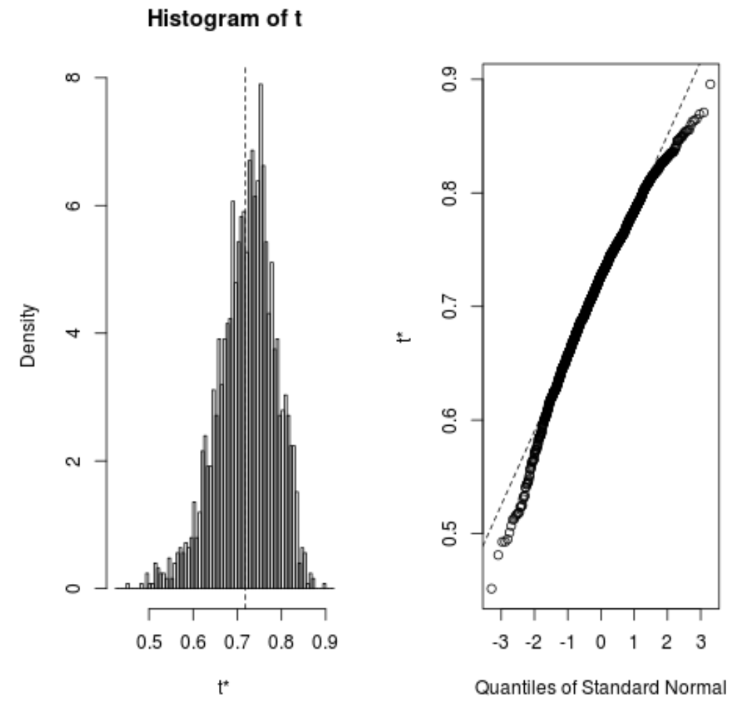
မော်ဒယ်၏ ခန့်မှန်းထားသော R-squared အတွက် 95% ယုံကြည်မှုကြားကာလကို တွက်ချက်ရန် အောက်ပါကုဒ်ကိုလည်း အသုံးပြုနိုင်ပါသည်။

 #calculate adjusted bootstrap percentile (BCa) interval
boot.ci(reps, type=" bca ")

CALL: 
boot.ci(boot.out = reps, type = "bca")

Intervals: 
Level BCa          
95% (0.5350, 0.8188)  
Calculations and Intervals on Original Scale

ရလဒ်မှ၊ စစ်မှန်သော R-squared တန်ဖိုးများအတွက် bootstrapped 95% ယုံကြည်မှုကြားကာလသည် (0.5350၊ 0.8188) ဖြစ်သည်ကို ကျွန်ုပ်တို့တွေ့မြင်နိုင်ပါသည်။

ဥပမာ 2- bootstrap များစွာသော စာရင်းအင်းများ

အောက်ဖော်ပြပါ ကုဒ်သည် များစွာသော မျဉ်းကြောင်း ဆုတ်ယုတ်မှုပုံစံတွင် ကိန်းဂဏန်းတစ်ခုစီအတွက် စံအမှားကို တွက်ချက်နည်းကို ပြသသည်-

 set.seed(0)
library (boot)

#define function to calculate fitted regression coefficients
coef_function <- function (formula, data, indices) {
  d <- data[indices,] #allows boot to select sample
  fit <- lm(formula, data=d) #fit regression model
  return (coef(fit)) #return coefficient estimates of model
}

#perform bootstrapping with 2000 replications
reps <- boot(data=mtcars, statistic=coef_function, R=2000, formula=mpg~disp)

#view results of boostrapping
reps

ORDINARY NONPARAMETRIC BOOTSTRAP


Call:
boot(data = mtcars, statistic = coef_function, R = 2000, formula = mpg ~ 
    available)


Bootstrap Statistics:
       original bias std. error
t1* 29.59985476 -5.058601e-02 1.49354577
t2* -0.04121512 6.549384e-05 0.00527082

ရလဒ်များမှ ကျွန်ုပ်တို့ မြင်နိုင်သည်-

• မော်ဒယ်ကြားဖြတ်အတွက် ခန့်မှန်းကိန်းသည် 29.59985476 ဖြစ်ပြီး ဤခန့်မှန်းချက်၏ စံအမှားမှာ 1.49354577 ဖြစ်သည်။
• မော်ဒယ်ရှိ ခန့်မှန်းတွက်ချက်မှု ပြောင်းလဲနိုင်သော disp အတွက် ခန့်မှန်းကိန်းဂဏန်းမှာ -0.04121512 ဖြစ်ပြီး ဤခန့်မှန်းချက်၏ စံအမှားမှာ 0.00527082 ဖြစ်သည်။

bootstrapped နမူနာများ ဖြန့်ကျက်မှုကိုလည်း လျင်မြန်စွာ မြင်ယောင်နိုင်သည်-

 plot(reps, index=1) #intercept of model
plot(reps, index=2) #disp predictor variable

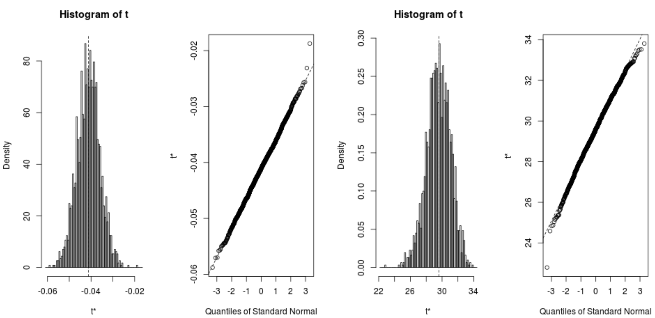
coefficient တစ်ခုစီအတွက် 95% ယုံကြည်မှုကြားကာလများကို တွက်ချက်ရန် အောက်ဖော်ပြပါ ကုဒ်ကိုလည်း အသုံးပြုနိုင်ပါသည်။

 #calculate adjusted bootstrap percentile (BCa) intervals
boot.ci(reps, type=" bca ", index=1) #intercept of model
boot.ci(reps, type=" bca ", index=2) #disp predictor variable

CALL: 
boot.ci(boot.out = reps, type = "bca", index = 1)

Intervals: 
Level BCa          
95% (26.78, 32.66)  
Calculations and Intervals on Original Scale
BOOTSTRAP CONFIDENCE INTERVAL CALCULATIONS
Based on 2000 bootstrap replicates

CALL: 
boot.ci(boot.out = reps, type = "bca", index = 2)

Intervals: 
Level BCa          
95% (-0.0520, -0.0312)  
Calculations and Intervals on Original Scale

ရလဒ်များမှ၊ မော်ဒယ် coefficients အတွက် bootstrapped 95% ယုံကြည်မှုကြားကာလများသည် အောက်ပါအတိုင်းဖြစ်သည်ကို ကျွန်ုပ်တို့တွေ့မြင်နိုင်သည်-

• ကြားဖြတ်အတွက် IC- (26.78၊ 32.66)
• disp အတွက် CI : (-.0520, -.0312)

ထပ်လောင်းအရင်းအမြစ်များ

R တွင် ရိုးရှင်းသော linear regression လုပ်နည်း
R တွင် linear regression အများအပြားလုပ်ဆောင်နည်း
Confidence Intervals နိဒါန်း