R တွင် spline regression ကို မည်သို့လုပ်ဆောင်ရမည်နည်း (ဥပမာနှင့်အတူ)

Spline regression သည် ဒေတာရှိပုံစံ ရုတ်ခြည်းပြောင်းလဲသွားပြီး linear regression နှင့် polynomial regression တို့သည် ဒေတာနှင့် အံဝင်ခွင်ကျမဖြစ်လောက်အောင် လိုက်လျောညီထွေဖြစ်စေသော အချက်များ သို့မဟုတ် “ အဖုများ” ရှိသည့်အခါ အသုံးပြုသည့် ဆုတ်ယုတ်မှုအမျိုးအစားတစ်ခုဖြစ်သည်။

အောက်ဖော်ပြပါ အဆင့်ဆင့် ဥပမာသည် R တွင် spline regression လုပ်ဆောင်ပုံကို ပြသသည်။

အဆင့် 1: ဒေတာကိုဖန်တီးပါ။

ဦးစွာ၊ variable နှစ်ခုဖြင့် R တွင် dataset တစ်ခုကိုဖန်တီးပြီး variables များကြားဆက်ဆံရေးကိုမြင်ယောင်နိုင်ရန် scatterplot တစ်ခုကိုဖန်တီးကြပါစို့။

 #create data frame
df <- data. frame (x=1:20,
                 y=c(2, 4, 7, 9, 13, 15, 19, 16, 13, 10,
                     11, 14, 15, 15, 16, 15, 17, 19, 18, 20))

#view head of data frame
head(df)

  xy
1 1 2
2 2 4
3 3 7
4 4 9
5 5 13
6 6 15

#create scatterplot
plot(df$x, df$y, cex= 1.5 , pch= 19 )

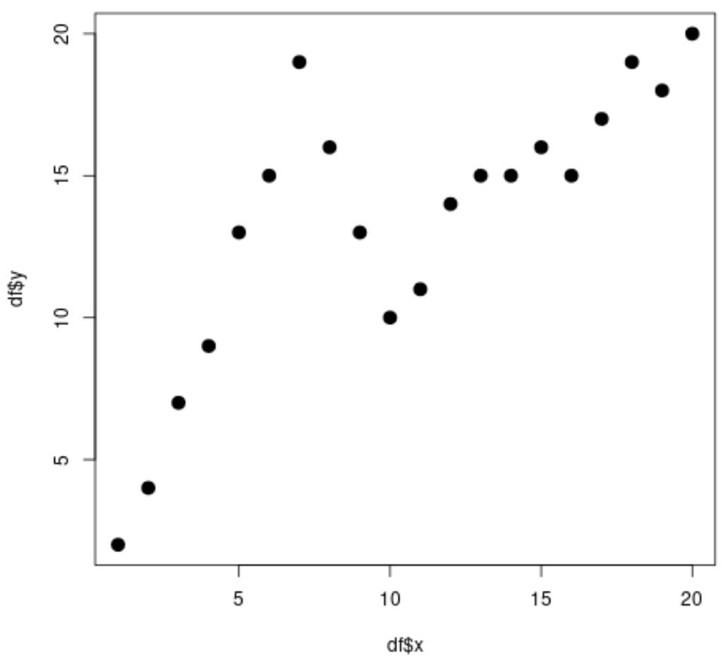
x နှင့် y အကြား ဆက်ဆံရေးသည် မျဉ်းမညီဘဲ ဒေတာရှိပုံစံသည် x=7 နှင့် x=10 တွင် ရုတ်ချည်းပြောင်းလဲသွားသည့် အချက်နှစ်ချက် သို့မဟုတ် “ nodes” ရှိပုံပေါ်သည်။

အဆင့် 2- ရိုးရှင်းသော linear regression model ကို ကိုက်ညီပါ။

ထို့နောက် ဤဒေတာအတွဲအတွက် ရိုးရှင်းသောမျဉ်းကြောင်းဆုတ်ယုတ်မှုပုံစံကို အံဝင်ခွင်ကျဖြစ်စေရန်အတွက် lm() လုပ်ဆောင်ချက်ကို အသုံးပြု၍ ကွက်လပ်ပေါ်တွင် ဆုတ်ယုတ်မှုမျဉ်းအား ကွက်ကွက်ကွင်းကွင်းပြုလုပ်ကြပါစို့။

 #fit simple linear regression model
linear_fit <- lm(df$y ~ df$x)

#view model summary
summary(linear_fit)

Call:
lm(formula = df$y ~ df$x)

Residuals:
    Min 1Q Median 3Q Max 
-5.2143 -1.6327 -0.3534 0.6117 7.8789 

Coefficients:
            Estimate Std. Error t value Pr(>|t|)    
(Intercept) 6.5632 1.4643 4.482 0.000288 ***
df$x 0.6511 0.1222 5.327 4.6e-05 ***
---
Significant. codes: 0 '***' 0.001 '**' 0.01 '*' 0.05 '.' 0.1 ' ' 1

Residual standard error: 3.152 on 18 degrees of freedom
Multiple R-squared: 0.6118, Adjusted R-squared: 0.5903 
F-statistic: 28.37 on 1 and 18 DF, p-value: 4.603e-05

#create scatterplot
plot(df$x, df$y, cex= 1.5 , pch= 19 )

#add regression line to scatterplot
abline(linear_fit) 

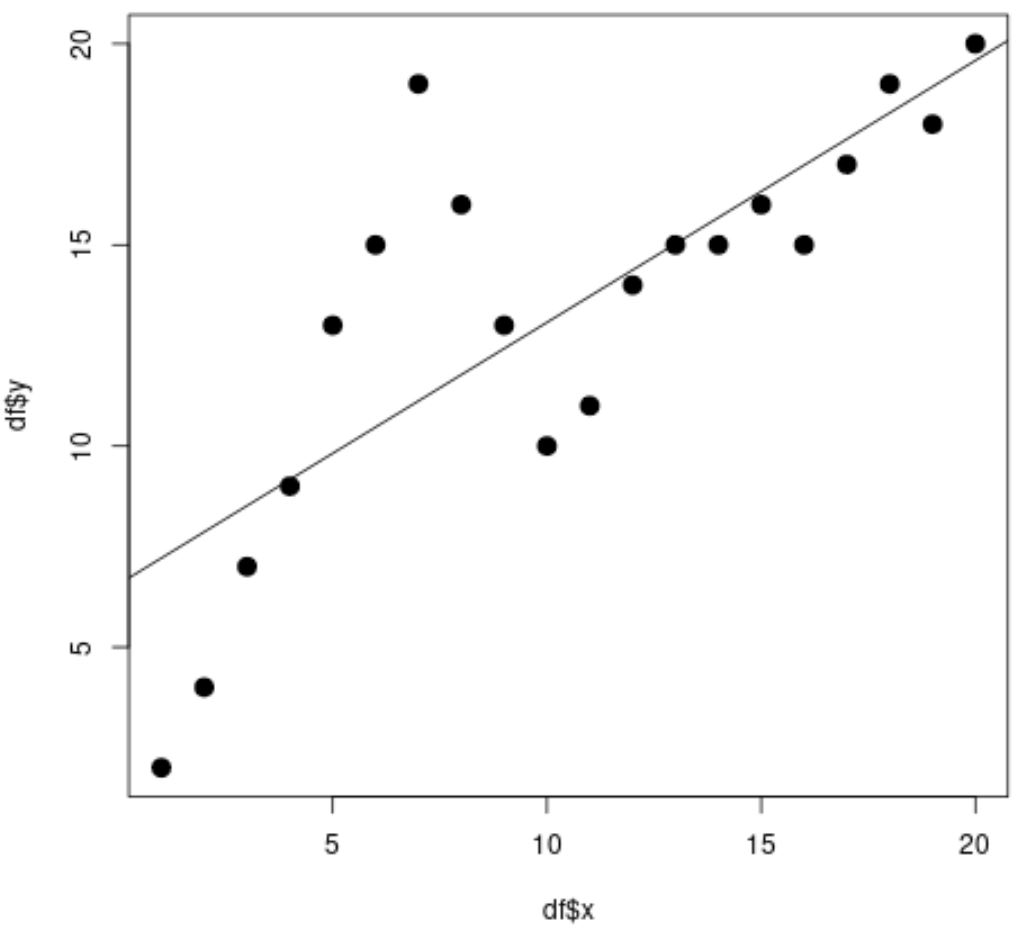
scatterplot မှ၊ ရိုးရှင်းသော linear regression line သည် data နှင့် ကောင်းစွာမကိုက်ညီကြောင်း ကျွန်ုပ်တို့တွေ့နိုင်ပါသည်။

မော်ဒယ်ရလဒ်များမှ၊ ချိန်ညှိထားသော R-squared တန်ဖိုး သည် 0.5903 ဖြစ်ကြောင်းကိုလည်း ကျွန်ုပ်တို့တွေ့မြင်နိုင်ပါသည်။

၎င်းကို spline မော်ဒယ်တစ်ခု၏ ချိန်ညှိထားသော R-squared တန်ဖိုးနှင့် နှိုင်းယှဉ်ပါမည်။

အဆင့် 3- spline regression model ကို အံကိုက်လုပ်ပါ။

ထို့နောက်၊ spline regression model ကို node နှစ်ခုနှင့် အံဝင်ခွင်ကျဖြစ်စေရန်အတွက် splines package မှ bs() function ကိုသုံးကာ၊ ထို့နောက် scatterplot တွင် တပ်ဆင်ထားသော model ကို ချရေးကြပါစို့။

 library (splines)

#fit spline regression model
spline_fit <- lm(df$y ~ bs(df$x, knots=c( 7 , 10 )))

#view summary of spline regression model
summary(spline_fit)

Call:
lm(formula = df$y ~ bs(df$x, knots = c(7, 10)))

Residuals:
     Min 1Q Median 3Q Max 
-2.84883 -0.94928 0.08675 0.78069 2.61073 

Coefficients:
                            Estimate Std. Error t value Pr(>|t|)    
(Intercept) 2.073 1.451 1.429 0.175    
bs(df$x, knots = c(7, 10))1 2.173 3.247 0.669 0.514    
bs(df$x, knots = c(7, 10))2 19.737 2.205 8.949 3.63e-07 ***
bs(df$x, knots = c(7, 10))3 3.256 2.861 1.138 0.274    
bs(df$x, knots = c(7, 10))4 19.157 2.690 7.121 5.16e-06 ***
bs(df$x, knots = c(7, 10))5 16.771 1.999 8.391 7.83e-07 ***
---
Significant. codes: 0 '***' 0.001 '**' 0.01 '*' 0.05 '.' 0.1 ' ' 1

Residual standard error: 1.568 on 14 degrees of freedom
Multiple R-squared: 0.9253, Adjusted R-squared: 0.8987 
F-statistic: 34.7 on 5 and 14 DF, p-value: 2.081e-07

#calculate predictions using spline regression model
x_lim <- range(df$x)
x_grid <- seq(x_lim[ 1 ], x_lim[ 2 ])
preds <- predict(spline_fit, newdata=list(x=x_grid))

#create scatter plot with spline regression predictions
plot(df$x, df$y, cex= 1.5 , pch= 19 )
lines(x_grid, preds) 

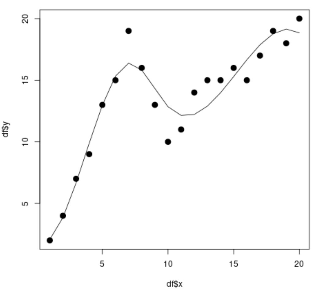
scatterplot မှ၊ spline regression model သည် data ကို အတော်လေး အံဝင်ခွင်ကျ လုပ်နိုင်သည်ကို တွေ့နိုင်ပါသည်။

မော်ဒယ်ရလဒ်များမှ၊ ချိန်ညှိထားသော R-squared တန်ဖိုးသည် 0.8987 ဖြစ်သည်ကို ကျွန်ုပ်တို့တွေ့နိုင်သည်။

ဤမော်ဒယ်အတွက် ချိန်ညှိထားသော R-squared တန်ဖိုးသည် ရိုးရိုး linear regression model ထက် များစွာပိုမိုမြင့်မားသည်၊ ၎င်းသည် spline regression model သည် data နှင့် ပိုမိုအံဝင်ခွင်ကျဖြစ်နိုင်ကြောင်း ကျွန်ုပ်တို့ကိုပြောပြသည်။

ဤနမူနာအတွက် node များကို x=7 နှင့် x=10 တွင်တည်ရှိကြောင်း သတိပြုပါ။

လက်တွေ့တွင်၊ သင်သည် ဒေတာရှိပုံစံများ ပြောင်းလဲပုံပေါ်ပြီး သင်၏ ဒိုမိန်းကျွမ်းကျင်မှုအပေါ် အခြေခံ၍ node တည်နေရာများကို သင်ကိုယ်တိုင် ရွေးချယ်ရန် လိုအပ်မည်ဖြစ်ပါသည်။

ထပ်လောင်းအရင်းအမြစ်များ

အောက်ဖော်ပြပါ သင်ခန်းစာများသည် R တွင် အခြားဘုံအလုပ်များကို မည်သို့လုပ်ဆောင်ရမည်ကို ရှင်းပြသည်-

R တွင် linear regression အများအပြားလုပ်ဆောင်နည်း
R တွင် exponential regression လုပ်ဆောင်နည်း
R တွင် အလေးချိန် အနည်းဆုံး စတုရန်း ဆုတ်ယုတ်မှုကို မည်သို့လုပ်ဆောင်ရမည်နည်း