R in curve fitting (ဥပမာများနှင့်အတူ)

မကြာခဏဆိုသလို R ၏မျဉ်းကွေးနှင့်အသင့်တော်ဆုံးညီမျှခြင်းကို သင်ရှာလိုပေမည်။

အောက်ဖော်ပြပါ အဆင့်ဆင့် ဥပမာတွင် poly() လုပ်ဆောင်ချက်ကို အသုံးပြု၍ R တွင် မျဉ်းကွေးများကို ဒေတာနှင့် အံဝင်ခွင်ကျဖြစ်အောင် ပြုလုပ်နည်းနှင့် မည်သည့်မျဉ်းကွေးသည် ဒေတာနှင့် ကိုက်ညီကြောင်း ဆုံးဖြတ်နည်းကို ရှင်းပြထားသည်။

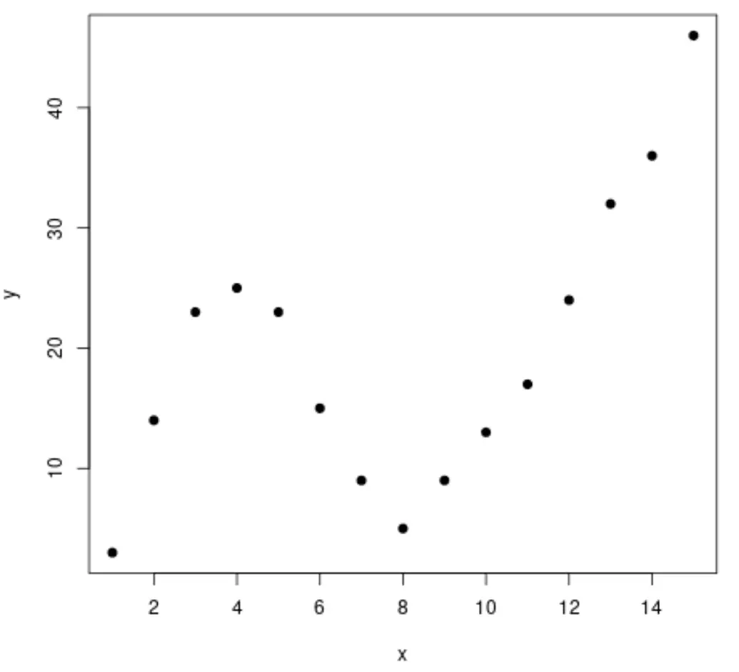
အဆင့် 1- ဒေတာကို ဖန်တီးပြီး မြင်ယောင်ကြည့်ပါ။

အတုအပဒေတာအတွဲကို ဖန်တီးပြီး ဒေတာကိုမြင်ယောင်နိုင်ရန် အပိုင်းအစတစ်ခုကို ဖန်တီးကြပါစို့။

 #create data frame
df <- data. frame (x=1:15,
                 y=c(3, 14, 23, 25, 23, 15, 9, 5, 9, 13, 17, 24, 32, 36, 46))

#create a scatterplot of x vs. y
plot(df$x, df$y, pch= 19 , xlab=' x ', ylab=' y ') 

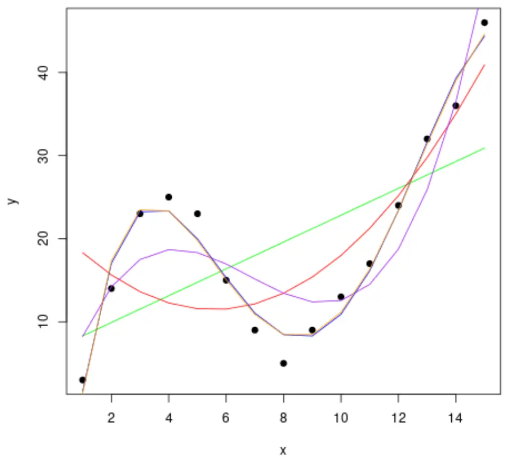
အဆင့် 2- မျဉ်းကွေးများစွာကို ချိန်ညှိပါ။

ထို့နောက် ကိန်းဂဏန်းများစွာကို ဆုတ်ယုတ်မှုပုံစံများကို ဒေတာနှင့် အံဝင်ခွင်ကျဖြစ်အောင် တူညီသောကွက်လပ်တွင် မော်ဒယ်တစ်ခုစီ၏ မျဉ်းကွေးကို မြင်ယောင်ကြည့်ကြပါစို့။

 #fit polynomial regression models up to degree 5
fit1 <- lm(y~x, data=df)
fit2 <- lm(y~poly(x,2,raw= TRUE ), data=df)
fit3 <- lm(y~poly(x,3,raw= TRUE ), data=df)
fit4 <- lm(y~poly(x,4,raw= TRUE ), data=df)
fit5 <- lm(y~poly(x,5,raw= TRUE ), data=df)

#create a scatterplot of x vs. y
plot(df$x, df$y, pch=19, xlab=' x ', ylab=' y ')

#define x-axis values
x_axis <- seq(1, 15, length= 15 )

#add curve of each model to plot
lines(x_axis, predict(fit1, data. frame (x=x_axis)), col=' green ')
lines(x_axis, predict(fit2, data. frame (x=x_axis)), col=' red ')
lines(x_axis, predict(fit3, data. frame (x=x_axis)), col=' purple ')
lines(x_axis, predict(fit4, data. frame (x=x_axis)), col=' blue ')
lines(x_axis, predict(fit5, data. frame (x=x_axis)), col=' orange ')

မည်သည့်မျဉ်းကွေးသည် ဒေတာနှင့် ကိုက်ညီကြောင်း ဆုံးဖြတ်ရန်၊ မော်ဒယ်တစ်ခုစီ၏ ချိန်ညှိထားသော R စတုရန်း ကို ကြည့်ရှုနိုင်ပါသည်။

ဤတန်ဖိုးသည် ခန့်မှန်းသူကိန်းရှင်အရေအတွက်အတွက် ချိန်ညှိထားသော မော်ဒယ်ရှိ ခန့်မှန်းသူကိန်းရှင်(များ) က ရှင်းပြနိုင်သည့် တုံ့ပြန်မှုကိန်းရှင်တွင် ကွဲလွဲမှုရာခိုင်နှုန်းကို ပြောပြသည်။

 #calculated adjusted R-squared of each model
summary(fit1)$adj. r . squared
summary(fit2)$adj. r . squared
summary(fit3)$adj. r . squared
summary(fit4)$adj. r . squared
summary(fit5)$adj. r . squared

[1] 0.3144819
[1] 0.5186706
[1] 0.7842864
[1] 0.9590276
[1] 0.9549709

ရလဒ်မှ၊ အမြင့်ဆုံးချိန်ညှိထားသော R-squared ပါသည့်မော်ဒယ်သည် ချိန်ညှိထားသော R-squared 0.959 ရှိသည့် စတုတ္ထဒီဂရီပိုလီနိုမီးယားဖြစ်သည်ကို ကျွန်ုပ်တို့တွေ့နိုင်သည်။

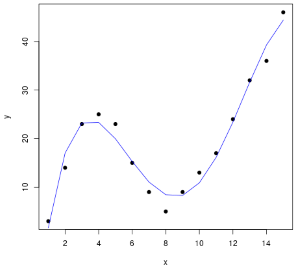
အဆင့် 3- နောက်ဆုံးမျဉ်းကွေးကို မြင်ယောင်ကြည့်ပါ။

နောက်ဆုံးတွင်၊ ကျွန်ုပ်တို့သည် စတုတ္ထဒီဂရီ ကိန်းဂဏန်းပုံစံ၏ မျဉ်းကွေးဖြင့် ဖြန့်ခွဲကွက်တစ်ခုကို ဖန်တီးနိုင်သည်-

 #create a scatterplot of x vs. y
plot(df$x, df$y, pch=19, xlab=' x ', ylab=' y ')

#define x-axis values
x_axis <- seq(1, 15, length= 15 )

#add curve of fourth-degree polynomial model
lines(x_axis, predict(fit4, data. frame (x=x_axis)), col=' blue ')

summary() လုပ်ဆောင်ချက်ကို အသုံးပြု၍ ဤစာကြောင်းအတွက် ညီမျှခြင်းကိုလည်း ရနိုင်သည်-

 summary(fit4)

Call:
lm(formula = y ~ poly(x, 4, raw = TRUE), data = df)

Residuals:
    Min 1Q Median 3Q Max 
-3.4490 -1.1732 0.6023 1.4899 3.0351 

Coefficients:
                         Estimate Std. Error t value Pr(>|t|)    
(Intercept) -26.51615 4.94555 -5.362 0.000318 ***
poly(x, 4, raw = TRUE)1 35.82311 3.98204 8.996 4.15e-06 ***
poly(x, 4, raw = TRUE)2 -8.36486 0.96791 -8.642 5.95e-06 ***
poly(x, 4, raw = TRUE)3 0.70812 0.08954 7.908 1.30e-05 ***
poly(x, 4, raw = TRUE)4 -0.01924 0.00278 -6.922 4.08e-05 ***
---
Significant. codes: 0 '***' 0.001 '**' 0.01 '*' 0.05 '.' 0.1 ' ' 1

Residual standard error: 2.424 on 10 degrees of freedom
Multiple R-squared: 0.9707, Adjusted R-squared: 0.959 
F-statistic: 82.92 on 4 and 10 DF, p-value: 1.257e-07

မျဉ်းကွေး၏ညီမျှခြင်းမှာ အောက်ပါအတိုင်းဖြစ်သည်။

y = -0.0192x ⁴ + 0.7081x ³ – 8.3649x ² + 35.823x – 26.516

မော်ဒယ်ရှိ ကြိုတင်ခန့်မှန်းကိန်းရှင်များကို အခြေခံ၍ တုံ့ပြန်မှုကိန်းရှင် ၏တန်ဖိုးကို ခန့်မှန်းရန် ဤညီမျှခြင်းအား ကျွန်ုပ်တို့အသုံးပြုနိုင်ပါသည်။ ဥပမာ x = 4 ဆိုရင် y = 23.34 ကို ခန့်မှန်းရပါလိမ့်မယ်။

y = -0.0192(4) ⁴ + 0.7081(4) ³ – 8.3649(4) ² + 35.823(4) – 26.516 = 23.34

ထပ်လောင်းအရင်းအမြစ်များ

Polynomial Regression နိဒါန်း
R တွင် Polynomial Regression (တစ်ဆင့်ပြီးတစ်ဆင့်)
R တွင် seq function ကိုအသုံးပြုနည်း