วิธีการคำนวณฟังก์ชัน sigmoid ใน python (พร้อมตัวอย่าง)

ฟังก์ชันซิกมอยด์ เป็นฟังก์ชันทางคณิตศาสตร์ที่แสดงเส้นโค้งรูปตัว “S” เมื่อพล็อต

ตัวอย่างที่พบบ่อยที่สุดของฟังก์ชัน sigmoid คือฟังก์ชัน logistic sigmoid ซึ่งคำนวณได้ดังนี้:

ฉ(x) = 1 / (1 + อี ^-x )

วิธีที่ง่ายที่สุดในการคำนวณฟังก์ชัน sigmoid ใน Python คือการใช้ฟังก์ชัน expit() จากไลบรารี SciPy ซึ่งใช้ไวยากรณ์พื้นฐานต่อไปนี้:

 from scipy. special import expit

#calculate sigmoid function for x = 2.5
expire(2.5)

ตัวอย่างต่อไปนี้แสดงวิธีใช้ฟังก์ชันนี้ในทางปฏิบัติ

ตัวอย่างที่ 1: คำนวณฟังก์ชันซิกมอยด์สำหรับค่า

รหัสต่อไปนี้แสดงวิธีการคำนวณฟังก์ชัน sigmoid สำหรับค่า x = 2.5:

 from scipy. special import expit

#calculate sigmoid function for x = 2.5
expire(2.5)

0.9241418199787566

ค่าของฟังก์ชันซิกมอยด์สำหรับ x = 2.5 คือ 0.924

เราสามารถยืนยันสิ่งนี้ได้โดยการคำนวณค่าด้วยตนเอง:

• ฉ(x) = 1 / (1 + อี ^-x )
• ฉ(x) = 1 / (1 + อี ^-2.5 )
• ฉ(x) = 1 / (1 + 0.082)
• ฉ(x) = 0.924

ตัวอย่างที่ 2: คำนวณฟังก์ชัน Sigmoid สำหรับหลายค่า

รหัสต่อไปนี้แสดงวิธีคำนวณฟังก์ชัน sigmoid สำหรับค่า x หลายค่าในคราวเดียว:

 from scipy. special import expit

#define list of values
values = [-2, -1, 0, 1, 2]

#calculate sigmoid function for each value in list
expire(values)

array([0.11920292, 0.26894142, 0.5, 0.73105858, 0.88079708])

ตัวอย่างที่ 3: การพล็อตฟังก์ชันซิกมอยด์สำหรับช่วงของค่า

รหัสต่อไปนี้แสดงวิธีการพล็อตค่าของฟังก์ชัน sigmoid สำหรับช่วงของค่า x โดยใช้ matplotlib :

 import matplotlib. pyplot as plt
from scipy. special import expit
import numpy as np

#define range of x-values
x = np. linspace (-10, 10, 100)

#calculate sigmoid function for each x-value
y = expire(x)
  
#createplot
plt. plot (x, y)
plt. xlabel (' x ')
plt. ylabel (' F(x) ')

#displayplot
plt. show ()

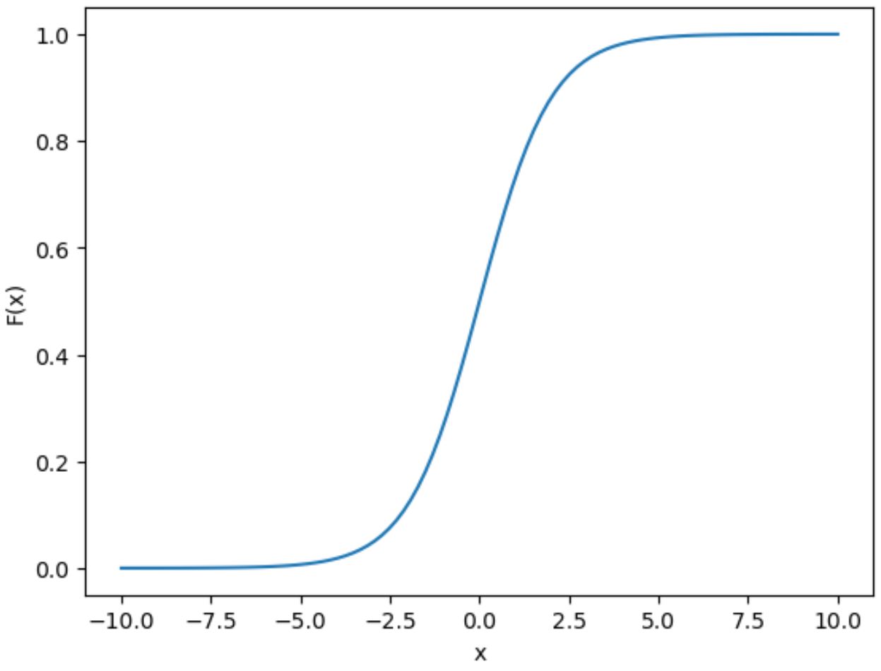
โปรดทราบว่าโครงเรื่องแสดงลักษณะเส้นโค้งรูปตัว “S” ของฟังก์ชันซิกมอยด์

แหล่งข้อมูลเพิ่มเติม

บทช่วยสอนต่อไปนี้จะอธิบายวิธีดำเนินการทั่วไปอื่นๆ ใน Python:

วิธีการดำเนินการถดถอยโลจิสติกใน Python
วิธีพล็อตกราฟการถดถอยโลจิสติกใน Python