Seaborn တွင် ဖြန့်ဝေနည်းကို ပုံဆွဲနည်း- ဥပမာများဖြင့်

ပင်လယ်မွေး ဒေတာမြင်ယောင်မှုပြစာကြည့်တိုက်ကို အသုံးပြု၍ Python တွင် တန်ဖိုးများဖြန့်ချီရန် အောက်ပါနည်းလမ်းများကို သင်အသုံးပြုနိုင်သည်-

နည်းလမ်း 1- histogram ကို အသုံးပြု၍ ဖြန့်ဖြူးမှုကို ပုံဖော်ပါ။

 sns. displot (data)

နည်းလမ်း 2- သိပ်သည်းဆမျဉ်းကွေးကို အသုံးပြု၍ ဖြန့်ဖြူးမှုကို ပုံဖော်ပါ။

 sns. displot (data, kind=' kde ')

နည်းလမ်း 3- histogram နှင့် density မျဉ်းကွေးကို အသုံးပြု၍ ဖြန့်ဖြူးမှုကို ပုံဖော်ပါ။

 sns. displot (data, kde= True )

အောက်ဖော်ပြပါ ဥပမာများသည် နည်းလမ်းတစ်ခုစီကို လက်တွေ့အသုံးချနည်းကို ပြသထားသည်။

ဥပမာ 1- Histogram ကို အသုံးပြု၍ ဖြန့်ဝေမှု အစီအစဉ်ဆွဲခြင်း။

အောက်ဖော်ပြပါ ကုဒ်သည် NumPy အခင်းအကျင်းတစ်ခုတွင် တန်ဖိုးများ ဖြန့်ကျက်ပုံကို ပင်လယ်ဖွားရှိ displot() လုပ်ဆောင်ချက်ကို အသုံးပြု၍ ပြသသည်-

 import seaborn as sns
import numpy as np

#make this example reproducible
n.p. random . seed ( 1 )

#create array of 1000 values that follows a normal distribution with mean of 10
data = np. random . normal (size= 1000 , loc= 10 )

#create histogram to visualize distribution of values
sns. displot (data)

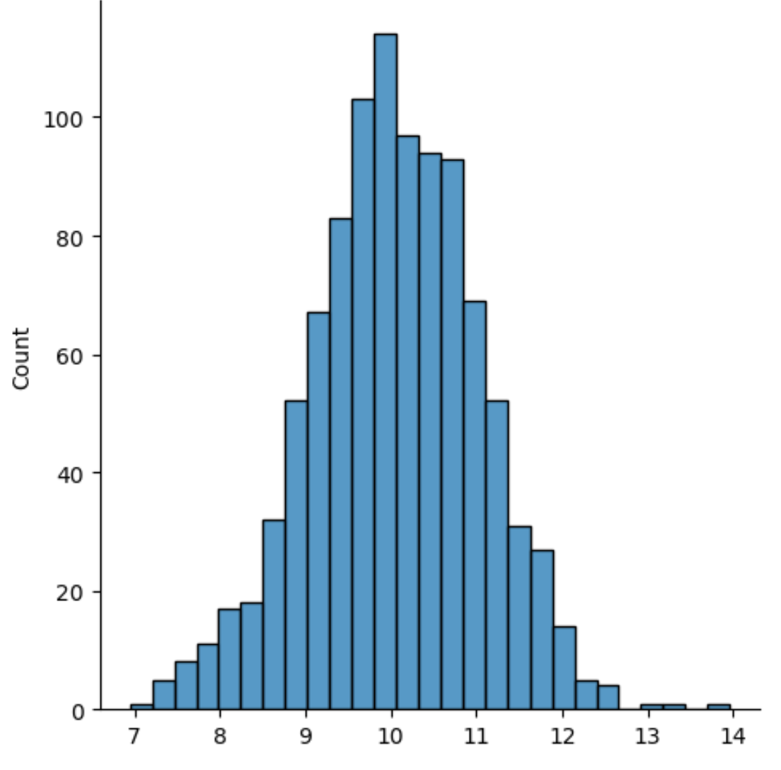
X ဝင်ရိုးသည် ဖြန့်ဖြူးမှုတန်ဖိုးများကိုပြသပြီး Y ဝင်ရိုးသည် တန်ဖိုးတစ်ခုစီ၏ရေတွက်မှုကိုပြသသည်။

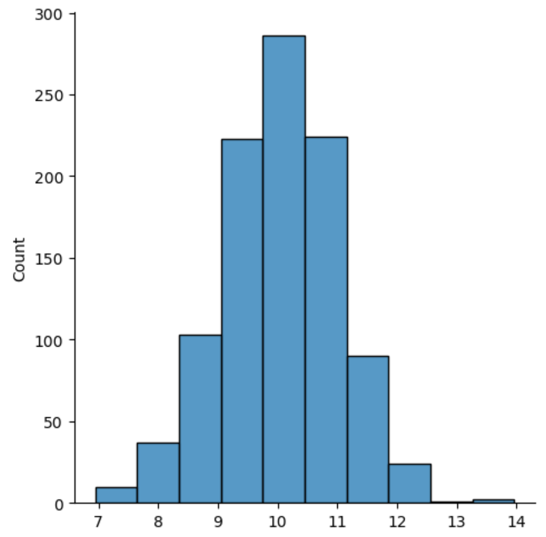
histogram တွင်အသုံးပြုသော bins အရေအတွက်ကို ပြောင်းလဲရန်၊ bins argument ကို အသုံးပြု၍ နံပါတ်တစ်ခုကို သတ်မှတ်နိုင်သည်။

 import seaborn as sns
import numpy as np

#make this example reproducible
n.p. random . seed ( 1 )

#create array of 1000 values that follows a normal distribution with mean of 10
data = np. random . normal (size= 1000 , loc= 10 )

#create histogram using 10 bins
sns. displot (data, bins= 10 ) 

ဥပမာ 2- Density Curve ကို အသုံးပြု၍ ဖြန့်ဝေမှုကို စီစဉ်ခြင်း။

အောက်ဖော်ပြပါ ကုဒ်သည် density မျဉ်းကွေးကို အသုံးပြု၍ NumPy အခင်းအကျင်းတွင် တန်ဖိုးများ ဖြန့်ဖြူးပုံကို ပုံဖော်နည်းကို ပြသသည်-

 import seaborn as sns
import numpy as np

#make this example reproducible
n.p. random . seed ( 1 )

#create array of 1000 values that follows a normal distribution with mean of 10
data = np. random . normal (size= 1000 , loc= 10 )

#create density curve to visualize distribution of values
sns. displot (data, kind=' kde ')

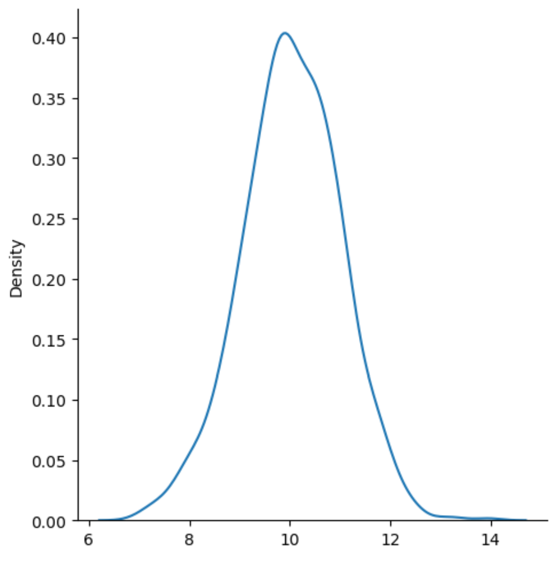
x-axis သည် ဖြန့်ဖြူးမှု၏တန်ဖိုးများကိုပြသပြီး y-axis သည် တန်ဖိုးတစ်ခုစီ၏ နှိုင်းရကြိမ်နှုန်းကိုပြသသည်။

type=’kde’ သည် kernel density ခန့်မှန်းချက်ကို အသုံးပြုရန် seaborn ကပြောသည်၊ ၎င်းသည် variable ၏တန်ဖိုးများခွဲဝေမှုကို အကျဉ်းချုပ်ဖော်ပြသည့်ချောမွေ့သောမျဉ်းကွေးကိုထုတ်ပေးသည်။

ဥပမာ 3- Histogram နှင့် Density Curve ကို အသုံးပြု၍ ဖြန့်ဝေမှုကို စီစဉ်ခြင်း။

အောက်ဖော်ပြပါ ကုဒ်သည် NumPy အခင်းအကျင်းတစ်ခုတွင် တန်ဖိုးများ ဖြန့်ကျက်ပုံကို စီစဥ်ထားသည့် သိပ်သည်းဆမျဉ်းကွေးတစ်ခုပါရှိသော ဟီစတိုဂရမ်ကို အသုံးပြု၍ ပြသသည်-

 import seaborn as sns
import numpy as np

#make this example reproducible
n.p. random . seed ( 1 )

#create array of 1000 values that follows a normal distribution with mean of 10
data = np. random . normal (size= 1000 , loc= 10 )

#create histogram with density curve overlaid to visualize distribution of values
sns. displot (data, kde= True )

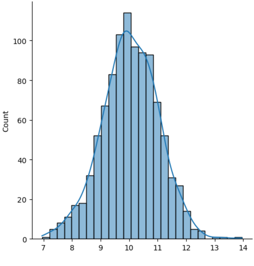
ရလဒ်မှာ သိပ်သည်းဆမျဉ်းကွေးကို တွဲထားသော ဟစ်စတိုဂရမ်တစ်ခုဖြစ်သည်။

မှတ်ချက် – seaborn displot() လုပ်ဆောင်ချက်အတွက် စာရွက်စာတမ်းအပြည့်အစုံကို ဤနေရာတွင် ရှာဖွေနိုင်ပါသည်။

ထပ်လောင်းအရင်းအမြစ်များ

အောက်ဖော်ပြပါ သင်ခန်းစာများသည် seaborn ကို အသုံးပြု၍ အခြားသော အလုပ်များကို မည်သို့လုပ်ဆောင်ရမည်ကို ရှင်းပြသည်-

Seaborn Plots တွင် ခေါင်းစဉ်တစ်ခုထည့်နည်း
Seaborn ကွက်များတွင် ဖောင့်အရွယ်အစားကို မည်သို့ပြောင်းရမည်နည်း။
Seaborn မြေကွက်များတွင် မှင်အရေအတွက်ကို ချိန်ညှိနည်း